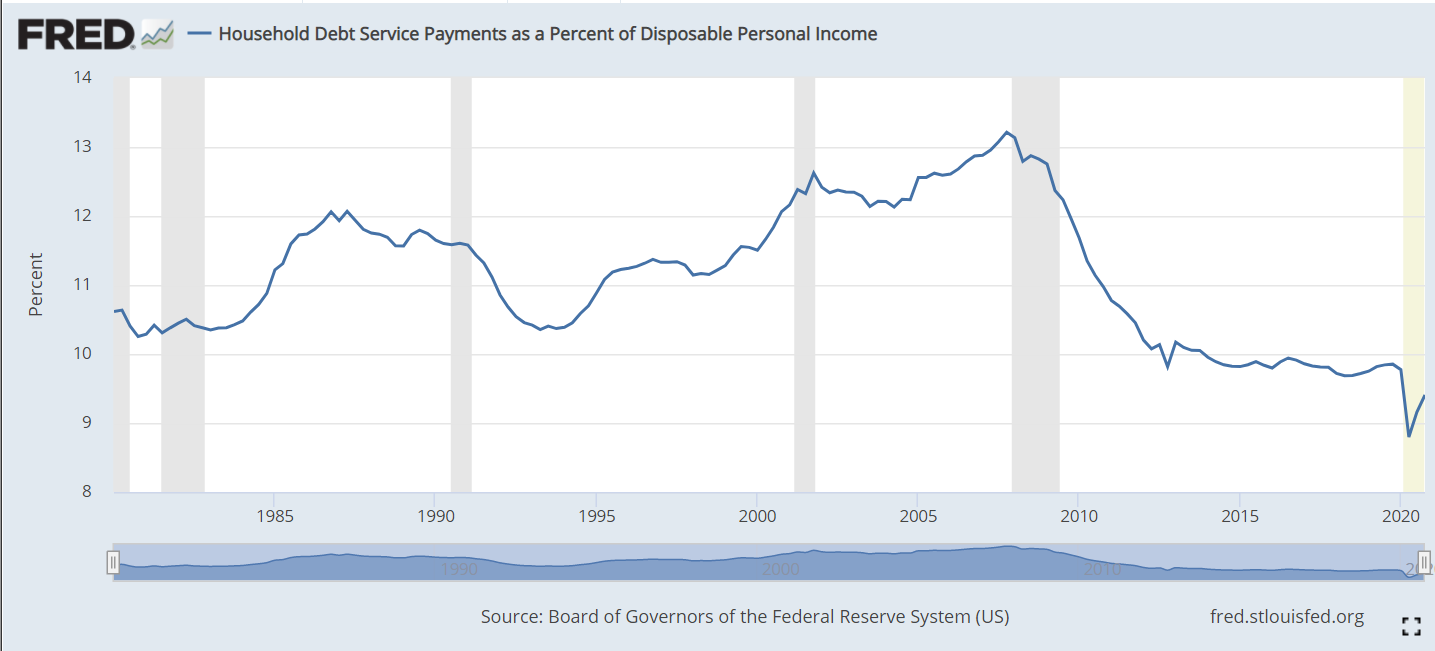
The ratio of household debt service (loan payments) to disposable personal income includes both mortgage payments and consumer debt payments. From 1980-2000 it fluctuated between 10.5% and 12%. Following the 2001 recession it increased to more than 13% before falling steeply to 10% in 2012. During the long recovery from the Great Recession it remained just below 10%. During the pandemic time it fell as low as 9% as personal incomes were boosted through stimulus payments. In total, this is a healthy situation. American families worked through an unsustainable runup of debt and payment during the “ought” decade, the Great Recession and the pandemic. They are well positioned at les than 10% to either save or spend, depending on their preferences. This is good news for the economy, the housing market and risks to financial markets. This is often called the Debt Service Ratio (DSR).
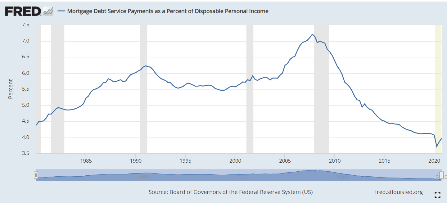
The mortgage component averaged 5.5% of personal income from 1980-2000. It remained below 6% through 2004, before increasing quickly to 7% in 2007. This was unsustainable. Mortgage foreclosures and revised lending standards reduced mortgage lending balances quickly. The Fed reduced interest rates and kept them low. Mortgage payments as a percent of disposable personal income fell to just above 4%. This is a 40% drop (3/7). Even compared with the 5.5% average, this is a 27% reduction in debt service expenditures. This ratio is threatened by future interest rate increases, but current mortgage holders will benefit from years of low mortgage rates and refinancing for decades to come.
Consumer debt has also fluctuated across these 40 years, reaching an early peak of 6.4% in 1986 during the confusing era of stagflation. In the next 6 years, families reduced their debt percentage by 1.7% to a safe minimum of 4.7%. Consumers were more confident through the 1990’s and took on more debt, allowing the payment ratio to rise to a new record of 6.6% before the 2000-2001 recession triggered less borrowing. Although mortgage payments increase during the 2000’s, consumer debt payments eased back to just 6.0%. Families were scared by the Great Recession and reduced their debt levels (and helped by lower interest rates) and payments to just 5% in 2010. The ratio remained low for 2 years, before resuming a familiar optimistic climb to 5.8% of disposable income before the pandemic.
The Household Financial Obligations Ratio (FOR) follows the same pattern as the Debt Service Ratio (DSR). It is a higher percentage as it includes other “fixed” obligations such as rent. We see relative stability between 16-17% through 2004. The mortgage driven increase to 18% by 2008 is evident, followed by a very rapid fall to 15% in 2012. This broader ratio has remained flat since then. The pandemic drop is due to extra stimulus income.
The composition of total consumer debt for the last 20 years highlights the rise and fall and rise of mortgage debt and the increase in student loan debt.
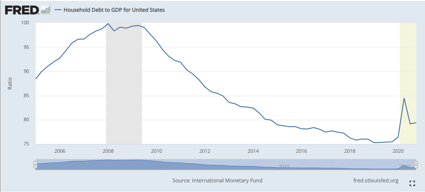
Household debt to GDP peaked at 100% before the Great Recession and has fallen by one-fourth in the next 10 years. Unpaid mortgages and other consumer debt have begun to accumulate in the last year.
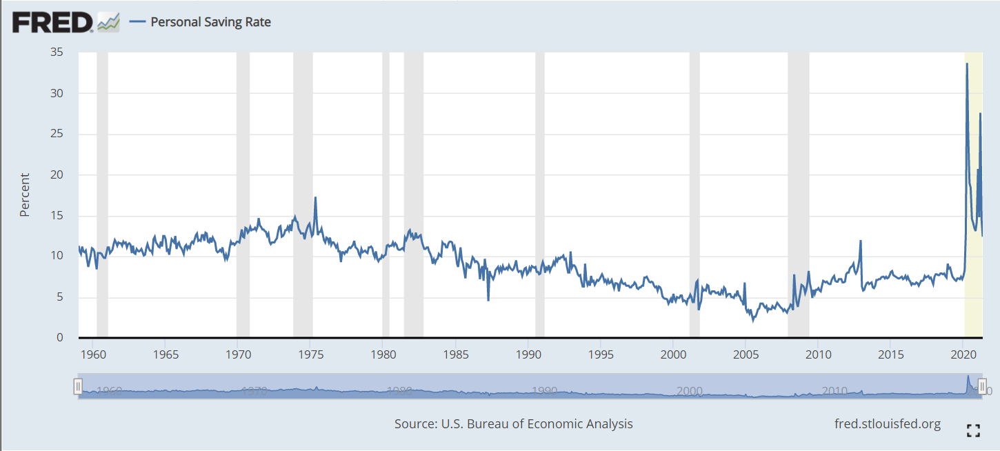
The personal savings rate averaged 10-13% from 1960-1985. The country’s economic challenges lead families to save less to maintain their standard of living, falling in half (5%) by 1999. It remained in the 4-5% range through the next expansion. The Great Recession triggered families to replenish their savings, with a 7-8% rate. The pandemic period shows a 15% savings rate. In all likelihood, this rate will fall back below 10% soon.
The overall US labor force participation rate is the ratio of those employed plus those actively looking for work among the non-institutional (military, prison, etc.) working age (16-64) population. It rose a quite substantial 8 points, from 59% in 1950 to 67% in 1990, mainly due to increased female participation rates. It remained in the 66-67% range through 2007, before declining by 5% in the last 14 years, a quite rapid decline. Note that the years selected are the ends of business cycle expansions plus the current year.
The overall rate mirrors the White rate as White’s make up the largest share of the population and because other racial participation rates are similar to the White rate. Black labor force participation has followed the White pattern, but been 2-3% lower than the White rate for most periods. The Hispanic rate started just below the White rate, but exceeded it by 1990, growing to a 3% advantage in 2021 at 65% versus 62%. The Asian participation rate has matched the White rate, sometimes being 1% higher.
The decline in the White share of the US population, especially in new births and school age children has been highly publicized and politicized for 40 years. The White share of the population has fallen from 5/6ths to just 3/5ths since 1950. African-American share grew by 2% in the 50’s and 60’s before settling at 12%. The Hispanic population has grown rapidly, from just 2% to 19%, passing the Black share by 2001. The broadly defined Asian population has grown from less than 1% to 6%. This breakdown does not include multi-race categories, which now amount to 3%. For labor force participation purposes, racial composition plays a minor role in the total rate.
Male participation in the labor force has fallen by 20 percentage points, from 87% to 67%. The increase in the 65+ age group from less than 4% to almost 8% of the total population accounts for more than 4% of this 20% decline, but 3/4ths or more is due to other factors. Female participation rates, working against this same 4% reduction due to the mix of older residents, grew from just 33% to a peak of 60% in 2001 before declining by 4%, about half of the male decline from 2001 to 2021. The expansion of opportunities for women and their choices to pursue the opportunities in the US is well understood. The increased share of aged 65+ women accounts for almost 3% of the 4% female decline. The reduction in male labor force participation is the big story.
Women, aged 55+ averaged just 22% participation through 1990. Most of the increased labor force participation in these 40 years was among younger women. More than one-third (35%) of women aged 55+ are now active labor market participants.
Their male counterparts in this age bracket show a 21 point decline, mirroring the overall male decline, but starting at the lower rate of 67% and ending at 46%. There is a mix variance here, as 55-64 year olds made up 4% of the population in the first 50 years, but now account for 6%, while the 65+ age group started at 4% for the first 25 years and then grew to 8%, so the share of 65+ citizens out of the 55+ total has risen from 45% to 56%. The mix variance accounts for a 5% decline in the participation rate, but the other 16% is due to other factors.
Demographers refer to the 25-54 year age group as the prime labor force. Here, we see women double their participation rate from 1950 (39%) to 2001 (77%) before falling off a bit to 74%.
For prime age men, we see a 9% point drop, from a near universal participation rate (97%) in 1950-60 down to 88% by 2018.
The White women data follows the total. A majority of Black women were labor force participants in 1970, 10 points higher than White women. They increased their labor force participation by 14 points, to a peak of 65% in 2001, before falling back by 5 points to 60% in 2021. This generally matches the pattern of White women, except that Black women have averaged an extra 4 participation points. Hispanic women started between the other two groups, at 45% in 1970 and then climbing to 60% in 2001. Their participation has remained close to 60%. Overall, relatively minor racial differences in female participation. About a 25 point increase in the second half of the 20th century followed by a 2 point decline in the last 20 years.
White men make up the largest share of the male total, so their data is close to the total, declining by 18 points, from 88% to 70%: from 7 out of 8 in the labor force to just 7 in 10. Black men follow the same Total pattern, but are consistently 4% less active in the labor market versus White men. Hispanic men first appear in the data in 1970, with an 85% participation rate, just above the 83% White male rate. However, Hispanic males stay at this level through 2007, while the White rate falls by 7%. In the last 14 years, the Hispanic male participation rate has dropped by the same 5% as the White and Black male rates, ending at 79%, 9 points above the 70% White rate.
Let’s start with the prime age labor force (25-54). From 1950 to 2001, we see a 19 point increase, from 65% to 84%. This is all due to the increase in female participation, which more than offset the significant decline in male participation. In total, from an economic point of view, this is great news. The total participation rate has slipped back a bit, from 84% to 81% in the last 2 decades, with men and women both falling back, but men falling faster. Aside from the distortion of the baby boom when it declined to 46%, the prime age group has typically been about 52-53% of the population. It has fallen by 1% in the last decade as the growth in older population groups has been faster than the decline in the childhood group.
The non-working age 0-15 year old childhood group reached a full 31% of the population total in 1960 and has since fallen to 19%. From an economic point of view, this too is good news, as the dependency ratio of non-workers to workers declines.
The teenager participation averaged 46% from 1950-1970. It averaged 55% in the mid-70’s to mid-90’s, but has quickly declined to just 34% in recent years. As teenagers make up 11% of the working age population, this drives a 2% decrease in the overall workforce participation rate. From an economic point of view, it is possible that the other activities of teens today are more valuable in creating human capital than the part-time entry level work that many more were performing in the 1970’s-90’s.
The labor force participation for young 20’s rose quickly from 64% to 77% by 1979 with increased participation by young women in the economy. The rate has declined to 70%. As this group accounts for 11% of the work age population, this has driven a nearly 1% point decrease in the overall work age participation rate.
The 55-64 year old group has a different pattern, averaging 61% in the 1950’s to 1970’s, decreasing 5 points to 56% in the mid-70’s through mid 90’s, before growing all the way back to 65% recently. The increased female participation rate did not impact this group significantly. During the 1975-95 time, more men took advantage of early retirement possibilities, some forced and some voluntary. This group increased from 9% to 12% of the total population. The 9 point participation rate increase since 1990 adds about one and one-half points to the overall participation rate, offsetting some of the 16-25 year old reduction.
The 65+ group pattern is similar to the 55-64 year olds, starting above 20%, falling down to 11% and returning to 20%. Economically, this recovery adds to the nation’s output, even if this group is not considered part of the work age population. This group has more than doubled as a share of the total population, reaching 15%.
With men and women combined, the total participation rate drops 5 points, from 67% in 2001 to 62% in 2021. The prime age group accounts for one-half of the working age population and shows a 3 point decline from 84% to 81%, with a one and one-half percent negative impact on the total rate. The significant declines in the 16-25 age group drives the rest of the 5 point decrease.
Data on labor force participation by educational attainment for ages 25-64 is available for 1970 through 2018. During this nearly 50 year period, the total participation rate increased from 70% to 79%, with a peak of 81% in 2001. Recall that the official total participation rate included the 16-24 year age brackets where participation fell significantly. We have only a 2 point decline from 2001 to 2018 rather than 5 points.
The big take-away is that participation rates for each group don’t change much through time. Those who didn’t complete high school average 61% pretty consistently. There are changes in the male and female participation rates and racial composition rippling through the data, but on average 3 of 5 people without a high school diploma participate in the labor market.
High school graduates average 76%, with a 3 point decline to 73% for 2018.
Individuals with some college classes have averaged 82% participation, except in 1970 when it was only 74%.
Those holding a college degree have averaged 86% participation, except in 1970 when they averaged 82%.
The proportion of citizens in each group has changed dramatically. Less than high school graduates dropped from 45% to just 10% of the post college working age population. College degree holders increased from11% to 35%. College attendees grew from 10% to 26%. High school grads started at 33%, increased to 38% and then declined to 29%. In total, the country shifted one-third of the population from non-high school education to college degree holders (BA and AA).
Given the consistency of labor force participation by level of educational attainment, the overall increase from 70% to 79% makes sense. Applying “typical” participation rates to each group (61.8, 74.5, 80.5, 85.7) produces an estimated participation rate for each year: 70, 73, 74, 77, 78 and 79. The 1990 and 2001 years stand out as having significantly higher actual than estimated labor force participation rates (+5 and +4). Perhaps some of the decrease in various rates since 1990 is due to there being an unusually high participation rate during this period as the economy expanded for relatively long periods with relatively mild recessions.
The prime age category is more than one-half of the labor force and contains individuals with the greatest earning power. Most attention has been focused on the 3 point drop from 2001 to 2021. It is also important to note the 19 point increase from 1950. We have data for men and women in this age group. Female participation essentially doubled from 1950 to 2001, before flattening out (down 2 points).
The male participation rate declines throughout the 70 year period, not just in the last 20 years. It falls from near universal 97% to 88%, meaning that 1 in 8 prime age males is not in the work force. As usually, the White rate matches the Total rate. Hispanic men have seen a 5 point decline from 1970-2018 while Whites fell 8 points. Hispanic men in 2018 had a higher participation rate than Whites. Black men started 7 points behind Whites at 90% and declined by an even larger 11% to just 79%. Whatever factors are driving prime age White men out of the labor force appear to be negatively impacting Hispanics and Blacks as well.
The overall participation rate for work age individuals (16-64) increased from 59% in 1950 to 67% in 1990 and has since dropped to 62%. The prime age group (25-54) increased from 65% to 84% before sliding back to 81%. For various age groups, the female participation rate doubled from mid 30 percent to high 60 percent range between 1950 and 2000 before slipping back a little. This drove the overall participation increase through 2001. The male participation rate for ages 16+ fell from 87% to 67% between 1950 and 2021. The prime age male (25-54%) rate dropped from 97% to 88%. Similar declines were seen for all races. The Obama white paper above (CEA) provides relevant details. The IBD article below is a good summary of this situation.
U.S. charitable giving to GDP ratio is 1.44%. Canada is second at 0.77%. UK is third at .54%. Italy at 0.3% is representative of Europe. U.S. giving is 5 times as high as other developed countries. (Table 27). U.S. private overseas aid is $44B. UK is second at $5B. (Table 25).
The World Giving Index has consistently rated the U.S. as the most generous country of 125 reviewed. Across 2010-19, US is 3rd highest percentage of those surveyed reporting they had “helped a stranger in the last year” at 72% compared with 48% global average. US was 5th highest with 42% reporting they had volunteered time for a charity in the past year versus 20% global average. US was 11th highest in percent reporting monetary donations in the last year (61%), versus global average of 30%.
In general, total US charitable giving has grown on a per capita or percent of GDP basis for more than 50 years. There is a clear “step up” in giving in the late 1990’s. Real (inflation adjusted) per capita giving has nearly doubled from representative $600 in 1970’s to $1,100 in 2000’s. (table 1). The US nonprofit sector reflects that growth, even though program fees are a much larger share of revenues, rising from less than 2% of GDP in the 1930’s-50’s to 3% in the 1970’s to more than 5% by the 2010’s. (table 6).
Total US charitable donations as a share of disposable income ratio has averaged roughly 2% across the last 40 years. Charitable giving as a percent of GDP averaged 1.7% in the 80’s and early 90’s, before increasing to 2.1% in the “oughts” and teens.
The most widely reported figure shows total real (inflation adjusted) US charitable giving since 1979. This has increased together with real US GDP. Representative years and amounts: 1982 ($150B), 1992 ($194), 2002 ($317), 2012 ($355) and 2019 ($450B).
Giving by individuals has fallen from 80% to 70% of the total. Bequests have increased from 7-8%. Foundation giving has more than doubled as a share of the total, from 7 to 16%. Hence, the real individual giving numbers are solid and rising, but their growth rate has slowed through time. 1982 ($130B), 1992 ($160), 2002 ($250), 2012 ($250), 2019 ($310).
While the total and individual charitable donation amounts have increased, the percentage of individuals donating has declined significantly. Years, percentages and average donation. 2002: 67%, $2,000. 2008: 65%, $2,300. 2012: 59%, $2,400. 2016: 53%, $2,500. Various authors speculate that the decline is caused by increasing inequality, lower confidence in institutions and changes in tax deduction laws.
In the early 2010’s there was a significant decrease in charitable giving percentages by non-itemizers (10%) and a much smaller decrease by itemizers (5%).
There are various reports that break down giving rates by state, city, religion, politics, region, marital status, generation and income. Perhaps most important is that the decrease in the giving percent from 67% to 53% means that the percentage giving zero, and dragging down the average, has increased from 33% to 47% of the population, from one-third to nearly one-half.
More than 90% of individuals with income above $125K donate to charity. 77% of those with incomes of $50-125K donate. This drops off to 58% at the $25-50K range and 37% under $25K (graph 11).
One source indicates that actual 2020 giving increased by 5%, with 1% more people making donations. This report also indicated that 23% of affluent donors increased their contributions to local projects and increased their unrestricted contributions.
Another source indicates that 2020 donations were up by 11% and the number of donors was up by 7%. They reported a 15% increase in small donations (<$250), an 8% increase in medium-sized donations and a 10% increase in large donation ($1,000+).
The US has a solid track record of individual charity. Donations have risen in real terms through time. Americans support nonprofits through cash and time donations. The decline in the percentage of individuals making donations is a concern. The “one-time” tax deduction for non-itemizing filers may help to spur increased contribution habits.
Peggy Noonan’s suggestion to use a 36 inch ruler to gauge right versus left in politics does help to explain the opposing views of tea partiers, Republicans and Democrats. Noonan describes 0 inches as pure right and 36 inches as pure left (opposite of what you might expect). She bemoans her perception that modern-day politicians negotiate between the 25 and 30 inch mark on the far left end of the ruler. She asserts that tea partiers will try to move back to the 5 inch mark.
In politics, he who sets the framework usually wins the game. Using American history since the agricultural 1770’s, urbanizing 1860’s, industrial 1920’s or depression 1930’s as a base, a case can be made that post-war politics and economics has been debated on the left end of the ruler, with a mixed economy government share of GDP at 20% and government spending/taxing share of GDP at 25-30%. These shares of the economy double those of laissez-faire capitalism, the roaring twenties or the depression. Noonan takes this long-run historical view of how the yardstick should be labeled.
Noonan is right in pointing out that politicians of both parties in a democratic system inherently seek to spend more money. The rise in government spending in the Bush presidency after the unusual decline in government spending in the Clinton presidency (with Republican congress) is a modern reminder. Tea partiers are right to have gut level concerns that government spending will continue to climb unchecked. The trend in 2000-2008 was up. Extraordinary banking and industry bail-out funds were piled on top of the stimulus spending for the Great Recession. Health care and social security spending increases are expected in the next two decades. Whether the various spending increases are justified or not, the trend is clearly up, without any clear countervailing force in Washington.
Those on the left might agree with the challenge to be faced, but they use a different scale to gauge left versus right, object to the accusation that they have driven up government spending, hold the Republicans responsible for inciting anger in the tea partiers and offer different long-run solutions.
If the scale is set between 100% individual, 0% government pure libertarianism versus 0% individual, 100% government pure socialism, the Democrats argue that the post-war game has all been played on the right (0-18 inch) side of the ruler. Government share of GDP is 20%. Government spending and taxes share of GDP is 30-35%, including all transfers. This did not increase between 1960 and 2008. The US tax burden at 27% of GDP is only 75% of the 36% average level for 30 developed countries. Only Mexico, Turkey, Korea and Japan spend less than the US. Total government spending in western European democracies is 40-55%. Government spending did increase with the Vietnam War and Great Society policies, but was reduced by the Reagan revolution. Government spending fell from 37.2% of GDP in 1992 to 32.6% in 2000.
Democrats argue that their fiscal discipline was demonstrated in 1992 to 2000 when they balanced the federal budget and reduced the deficit, employing the “pay as you go” policy to force spending cuts to offset spending increases. They point to Bush led Medicaid and defense spending increases as the cause of increased government by 2008. They see the Bush tax cuts as redistribution to the wealthy and don’t see the overall tax-cut initiated economic growth claimed to increase net tax revenues.
Democrats argue that they have not purposely increased the long-run share of government in the economy. They claim that the one-time investments/guarantees for the banking/auto industries were necessary for the whole economy, addressed issues that had grown for decades, will be partially recaptured and do not require continued funding. Similarly, they pursued a moderate one-time Keynesian fiscal stimulus in response to a deep recession, just as was done by other governments of all parties in all countries for the last 60 years. The stimulus spending lies between the 4.7% of GDP boost in 1982 and the 2.3% growth in 1992. Democrats argue that these actions are necessary and moderate and would have been undertaken by a responsible Republican successor to the Bush administration.
Democrats argue they are unfairly characterized as “big spenders” by the Republicans. This simple accusation has stirred a populist response from “regular Americans”. While Democrats have historically focused populist rage on big business and big banking, the Republicans and tea partiers have effectively used big government, Washington, elites, foreign countries and religions as targets, tying them to the Democratic Party. Democrats argue that the monetarist, supply side, tax cut economic policies of the Republican Party since Reagan have been adopted for their populist simplicity and political effectiveness alone, further polarizing economic policy making.
Finally, Democrats have adopted part of the Republican play book in fundamentally looking to the private sector to drive the future economic growth required to support even the historic level of government spending. The stimulus spending was partially focused on future industrial growth and infrastructure. The banks and auto firms are returning to pure private ownership. Small business lending and investment tax credits have become a focus. Health care reform maintained private providers and insurers as the core of the system. The costs of the war in Iran have been reduced. A bipartisan group has been appointed to work on the Medicare/social security future. Steps are being taken to promote exports. A reduced public sector role for the mortgage industry has been proposed. Obama and many Democrats have continued the pro-business approach used by Clinton.
On the other hand, Republicans can fairly point to steps taken by the Democrats that indicate a continued desire to “tax and spend”. The stimulus bill benefited state government, construction and other Democratic interests disproportionately. Health care reform achieved growth in government commitments without structural cost solutions. Labor unions were given special treatment in the auto bail-out. Fannie Mae and Freddie Mac’s roles were not touched in the banking reform. The financial consumer protection agency smacks of unlimited and uninformed regulation. The proposed increase in taxes for high earners is significant and is not coupled with structural spending reforms. A second mini-stimulus has been approved and unemployment benefits have been extended to record lengths.
The current economic situation has raised the stakes for politics. We should expect to see ongoing attempts to define the ruler and place the participants at marks that favor one group or another in the public eye.
The Bush administration experienced a weak jobs recovery from 2002-2007 and the Obama administration is facing even stronger headwinds in 2009-2010. Are there structural factors that are more important than the widely discussed business cycle and macroeconomic policy factors?
On the labor supply side, the growth of internet based job applications processes has greatly improved the effective supply of high quality candidates for all positions. This increases the expectation of firms of finding great fit candidates. On the other hand, until recently workers had inflexible wage expectations due to worker experience, pride, assets and family income alternatives. The decline in family housing and investment assets together with the greater experience of long-term unemployment has recently increased the willingness of potential employees to be flexible in seeking work. Human resources departments remain reluctant to greatly reduce hiring wages in fear of turnover, legal and internal equity challenges.
Extended unemployment benefits reduce the incentive to find work for some individuals, but this has a relatively minor labor supply impact.
Much greater structural changes have been experienced on the demand side of the equation. Perhaps most important has been the ongoing growth in labor productivity, which has reduced the effective demand for incremental employment. Increased staff flexibility in working long hours has also reduced the demand for peak-time or just in case workers
Firms have become more aggressive and experienced in downsizing employee groups as dictated by business conditions, thereby reducing the demand for labor. This could eventually result in greater future employment demand, since the expected future cost of maintaining partially productive staff is reduced. It appears that this cost reduction has been offset by a greater awareness that hiring an employee is a long-term investment decision. Firms that have been trying to rework the employment bargain from one of life-time loyalty to one of “fair dealing” remain very reluctant to plan for future downsizing, so they have set higher new staff addition thresholds, subject to the sensitivity analysis once reserved for major capital investments.
Firms have also become more aware of the all-in cost of hiring. Health care benefits costs per employee have increased significantly, especially as a percent to wages for hourly and entry-level jobs. Internet application processes have increased hiring costs for many firms. The level of firm-specific training required for break-even in many jobs has increased. With better models of hiring, firms are less willing to hire “good enough” candidates who do not fully meet all functional, industry, character and culture needs, resulting in positions which remain open for longer periods. Overextended managers have less incentive to add permanent positions. Firms are also less likely to invest in entry-level professional staff positions due to the higher turnover and lack of investment returns.
Labor force reductions have escalated in the last decade. Downsizings are conducted when indicated, even in times of plenty. Marginally productive or engaged staff members are moved up or out sooner. Employees in obsolete functions see their jobs eliminated. Protected functions or industries are quite rare today. In a labor intensive business world, firms are more aggressive in pairing staff.
Productivity improvement projects have become less labor investment intensive. Much improvement comes from getting more value out of the existing resources. The declining role of physical capital creates fewer tag along positions. Firms have learned to manage peak seasons and major projects with less incremental staffing. Information technology investments had stimulated some new forms of project and analytical staff needs in the last 30 years, but that demand is flat today. Firms have adopted standard process and project management templates that reduce the demand for new positions to accompany IT investments.
Firms are now fully aware of the use of contractors, part-time staff, consultants, outsourcing and imports to fill most functions. The need to hold partially employed staff is greatly reduced. Many processes have been re-engineered specifically to allow outsourced resources to be used to accommodate peak demands.
Finally, overall business investment has been weak in the post Y2K period. Firms have learned to manage inventories much better. They have installed significantly higher project hurdle rates based upon their experience with project failures. The lower market cost of capital has been a very minor factor outside of industries like real estate and banking. Through productivity improvements, the effective capital stock has increased without as much new investment. Sensitivity to the risks of change has caused firms to reduce the number of minor investment projects.
Business investment has been especially weak in the last 3 years, with firms freezing capital expenditures until the overall economic climate is resolved. This includes fiscal, monetary, trade, tax and regulation policies. The credit crunch has reduced hiring by small firms.
In general, firms have become much more effective in managing their capital, inventory, technology, brand and labor resources. Many of these changes in the last decade have reduced the demand for labor. Some of these changes may have a long-term impact on the minimum or natural unemployment rate, while others will cycle through business profits to business investment to increased labor force demand in the long-run.
Dow 35,000 was a dream in the go-go 1990’s when the new economy had supposedly broken all of the old rules. Dow 3,500 was a distinct fear in March, 2009 when stocks had fallen by more than half from their peak. Dow 10,000 is the most visible reference point in the current stock market.
Every investor and business degree holder knows that stock values are fundamentally based on the expected risk-adjusted net present value of future after-tax cash flows. They are also tempted by the “efficient markets hypothesis” that says that stock valuations incorporate all information about future returns and therefore set the present value in a rational manner. On the other hand, they understand fluctuations, random walks, animal spirits and the history of under and over valued stock markets.
Individuals who believe that stocks return 7-8% on average in the long-run through 2-4% dividend yields and 4-6% price increases, must conclude that the stock market is inherently irrational. It has been 30% undervalued or overvalued a majority of the last 100 years. Overvalued 1922-31. Undervalued 1932-54, except for 1936-37. Undervalued 1974-86. Overvalued 1996-2008.
Stocks were overvalued by 137% in 1929 before tumbling to -67% undervalued in 1933. Stocks reached an undervaluated low of -58% in 1942. Stocks reached a new -50% undervaluation during the depths of the 1982 recession. In 15 short years, by 1997, they reached a 57% overvaluation. They rose to 115% overvalued in 2000, before retreating to a mere 38% overvaluation in 2003. In 2008, stocks were 67% overvalued compared with the long-run trends.
Based on 100 years of history, the Dow Jones Industrial Average at the end of 2010 should be 9,000. The expected value in 2020 is 15,700, providing a 5% annual valuation return and 2% dividend return. Investors who bet against long-term average valuations do so at their own risk.
From sunbelt Florida to Georgia to Texas the local hiring reports remain negative for college grads for the second straight year.
When engineering students can’t find jobs, you know there’s a major problem.
When the Wall Street Journal writes about white collar parents and unemployed children, you know there’s a major problem.
The recovery graph in the latest Economist article shows that recovery is far slower than in past recessions.
Only the US News & World Report headline writer could find a way to put a positive spin on the situation with “Rosier Job Outlook for College Grads”, but even they recognized that “the job market remains treacherous for college grads”.
Net job creation finally turned positive last month. The leading economic indicators have been positive for 12 months in a row. Some reports, like record 27% housing sale increases, are “off the charts” positive, even if driven by an expiring tax credit.
Nonetheless, this will be a slow recovery. The 2002-2008 recovery was panned as the jobless recovery. Historically, financial crises require significant time to heal. The overextended American consumer, government, banks and dollar need time to adjust. The flexible US workforce has responded by increasing productivity by 6%, reducing the need to hire. Corporations budgeted for capital projects and new hires in 2010, but have not yet released the funds.
Like “the little engine who could”, it will take time for this economy to build up a head of steam. As the economy recovers, hiring will increase and employers will welcome those new college grads to cost-effectively replace those retiring Baby Boomers whose investments have gained 70% in the last year.
The U.S. labor market remains mired in a post WWII land of large employer paternalism that is unsuited to the needs of global competition. Major changes to labor laws should be made to lower the full costs of hiring employees. At the same time, major changes to unemployment insurance should be made to provide a meaningful safety net, without reducing the incentives for the unemployed to actively seek re-employment, even at lower wages when needed.
In return for a variety of actions to reduce the unit cost of labor by more than 20%, employers should be required to fund one-half of an unemployment insurance fund that provides meaningful benefits. Employees would fund the other half through payroll deductions. Unemployed workers would receive an initial payment of one-half of six months’ worth of wages. Additional 50% payments would be made at the beginning of third and fourth quarters of unemployment. This lump-sum approach maintains the incentive to actively seek new employment, while providing a true safety net in a world where 6 month bouts of unemployment are recurring career experiences at all levels.
The federal government could lower the transaction costs of employment by maintaining a national ID card system that qualifies individuals for employment and removes the hiring cost and risk to employers. The federal government could certify 3-5 firms to operate a standardized resume/profile system that records and certifies the basic education and employment history for individuals in one place.
Employees would be more attractive to employers if they invested more in their professional skills. A continuing education tax credit would improve candidate skills and remove the need for employers to offer most internal training and educational benefits.
Employers would hire more individuals if the terms of employment were more flexible. Labor laws could more clearly allow “paid time off” banks to be used in place of overtime compensation. The trigger for required overtime premiums could be raised from 40 to 48 hours for the first 10 weeks of annual overtime. Seasonal positions could be exempted from employer unemployment compensation responsibility. A new employment category could be created to clearly allow 100% incentive based sales positions. The IRS rules defining employees and contractors could be simplified to reduce administrative costs and risks.
Federal labor laws and regulations could be simplified to reduce administrative costs and limits could be placed on potential liabilities. The equal employment opportunity, family medical leave, disability and other employee “rights” acts incentivize employers to take extreme defensive steps and avoid hiring in order to avoid potential liabilities.
The federal government could incentivize the creation of new positions directly by paying half of the first six-months of wages. The rules for unpaid internships could be clarified, allowing students to work up to 700 hours per year within win-win educational programs which lead to employment. The labor laws could be clarified to allow “no fault” dismissals within 180 days.
In a globally competitive environment, labor laws need to benefit employers and employees. Steps can be taken to reduce the total cost of employment and protect employed and unemployed workers. The cost to employers and society through taxes is modest.
In addition to macroeconomic steps to improve the economy and administrative steps to provide meaningful unemployment compensation benefits and lower employment costs and risks, the federal government could change tax policies to significantly reduce the incremental costs of employing workers.
The federal government could incentive continuing education through tax credits. Unemployment compensation insurance could be shared by employers and employees. Family medical leave benefits could be funded by the federal government as is done in other developed nations.
Tax changes could be made to incentivize individuals to invest in their own life and disability insurance plans. Tax credits could be used to promote individual charitable contributions and reduce the need for corporate gifts and matching programs. The dollar and percentage limits for tax –deferred retirement plan contributions could be raised, increasing the value of compensation. The rules for qualified plans could be modified to allow a greater share of “highly compensated” employee pay to be made on a pre-tax basis.
Finally, the two biggest fringe benefits – social security and health benefits – could be migrated to government and employee funded programs over a decade, releasing employers from this responsibility. Social security can be funded from federal income tax revenues or simply made employee deduction. Health care insurance programs could lose their tax-deductible status. If no better option is found, employer contributions to consumer choice (HAS/HRA) plans could retain their tax-deductible status.
Allowing American employers to focus on creating jobs, operating their firms and making money will unleash incentives to increase productivity, competitiveness and our standard of living. Finding the political will to fund desired public services will not be easy, but the total benefits justify the short-term challenges.
It’s time to place some bets on the recovery. Buy low and sell high.
The labor market is softer than it has been since 1982. It’s time to act.
0. Reset the terms of employment with staff. Reduce health care, pension and other benefits to a sustainable level. Increase the share of incentive versus base compensation. Hire some support staff to avoid burnout. Offer a nominal pay increase now. Provide extra time and flexibility to staff to balance.
Hire qualified director/VP level staff to lead “on hold” initiatives. They are available for lower base compensation and are highly motivated to earn incentives.
Identify the most qualified scientific and technical staff in key R&D and product development areas. They are unable to obtain venture capital support and would welcome a paycheck or contract.
Complete your quality staffing, training and initiatives. The market is loaded with very highly qualified individuals who have the business savvy to deliver value.
Most suppliers are in weak positions, eager to begin to make progress.
0. Propose long-term agreements with key supplier partners in return for a 5% per year reduction in unit costs. Negotiate to a win-win position. The best partners can reduce costs every year. Focus on professional services firms. Legal, accounting, insurance, HR and real estate firms face a new reality of lower revenues and profits. They are ready to negotiate to maintain business.
Take another look at outsourcing areas that are not strategic core competencies. The third-party providers are more effective than ever and eager to do business. All of the line and staff areas should be reviewed: customer service, finance, accounting, HR, marketing, purchasing, logistics, distribution, manufacturing, and R&D.
Engage contingency based cost saving consultants. They are eager for business and can do their work with limited time from your staff.
Look at domestic suppliers of key products and components. The dollar is falling. Transportation and environmental costs are rising. Inventory and stock out opportunity costs are rising. The remaining domestic manufacturers have outstanding capabilities.
Make a few strategic investments.
0. The real estate market is very weak. Re-negotiate existing leases. Look at sale and lease back deals. Lease or secure options on properties for the future. Hire or contract for unemployed real estate experts to reduce total costs of facilities and their associated risks and taxes.
Take out those IT investment project lists. Invest in the high ROI projects. IT firms are ready to bargain, especially for larger, long-term deals. Consider applications like Microsoft Sharepoint that knit together web, sales and communications.
Pursue strategic acquisitions to acquire market share, products or talent. Equity values have recovered. Debt for solid larger firms is becoming available at low rates. Smaller and highly leveraged firms are nearing the end of their liquidity options and need to sell.
Pursue market share.
0. Strategically evaluate the structure, number and incentives of your sales force. You’ve maintained market share for the last 2 years. Remove low performers. Revise incentive schemes. Invest in sales training for younger staff. Make sure that your sales management team is the best possible. Hire strong performers from the real estate, banking and insurance industries.
Invest in export sales opportunities. The markets are growing. The dollar is falling. The infrastructure is available to get started with a lower initial investment.
Obama to unveil offshore drilling plans for oil, natural gas
The proposal through 2017 will open new areas of the mid-Atlantic region, Alaska and the eastern Gulf of Mexico for production but prohibit moves off California, Oregon and Washington.


