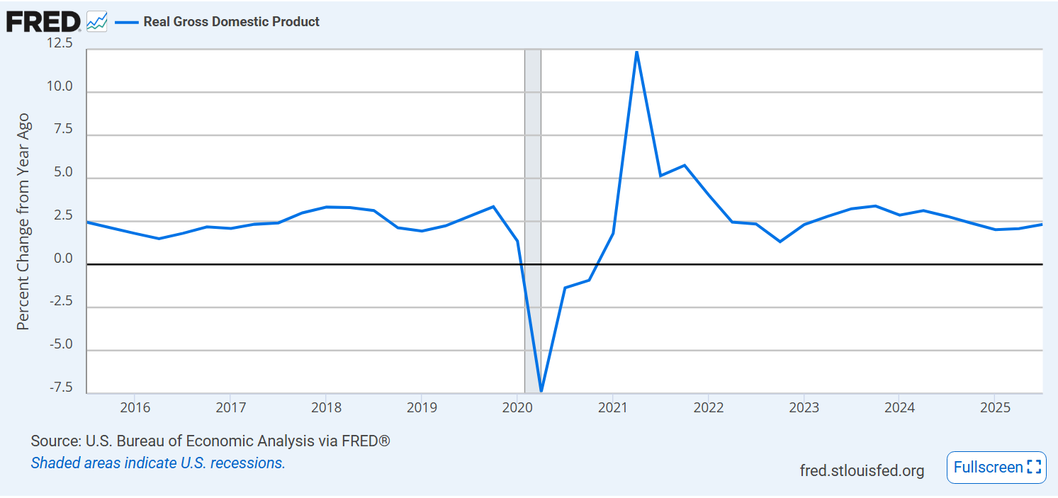
Overall, at the same core 2.5% growth rate seen for the last decade.
Labor productivity growth down a bit from the pandemic recovery bump.
Median wage growth remains at 2%, down a bit from pre-pandemic 2.5%.
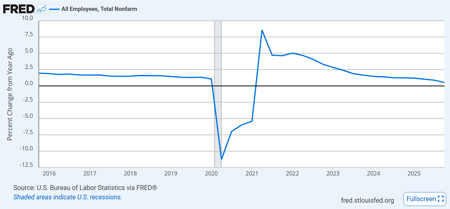
Job growth is very weak. Typically, this indicates a coming recession, but the reduction of the immigration labor supply makes historical comparisons difficult.
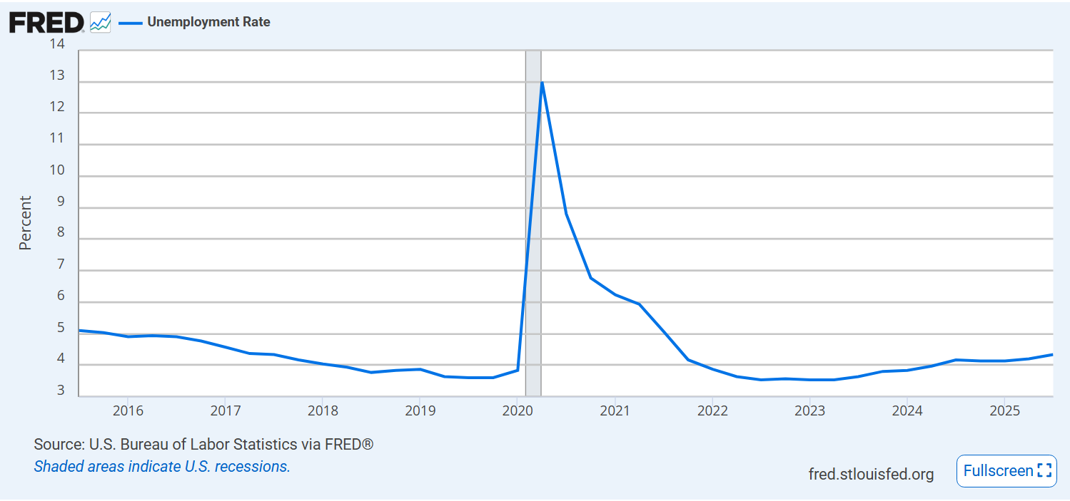
Unemployment rate remains at historically low 4.5% but it has been increasing for more than 2 years.
The “underemployed” rate shows the same relative level and trend.
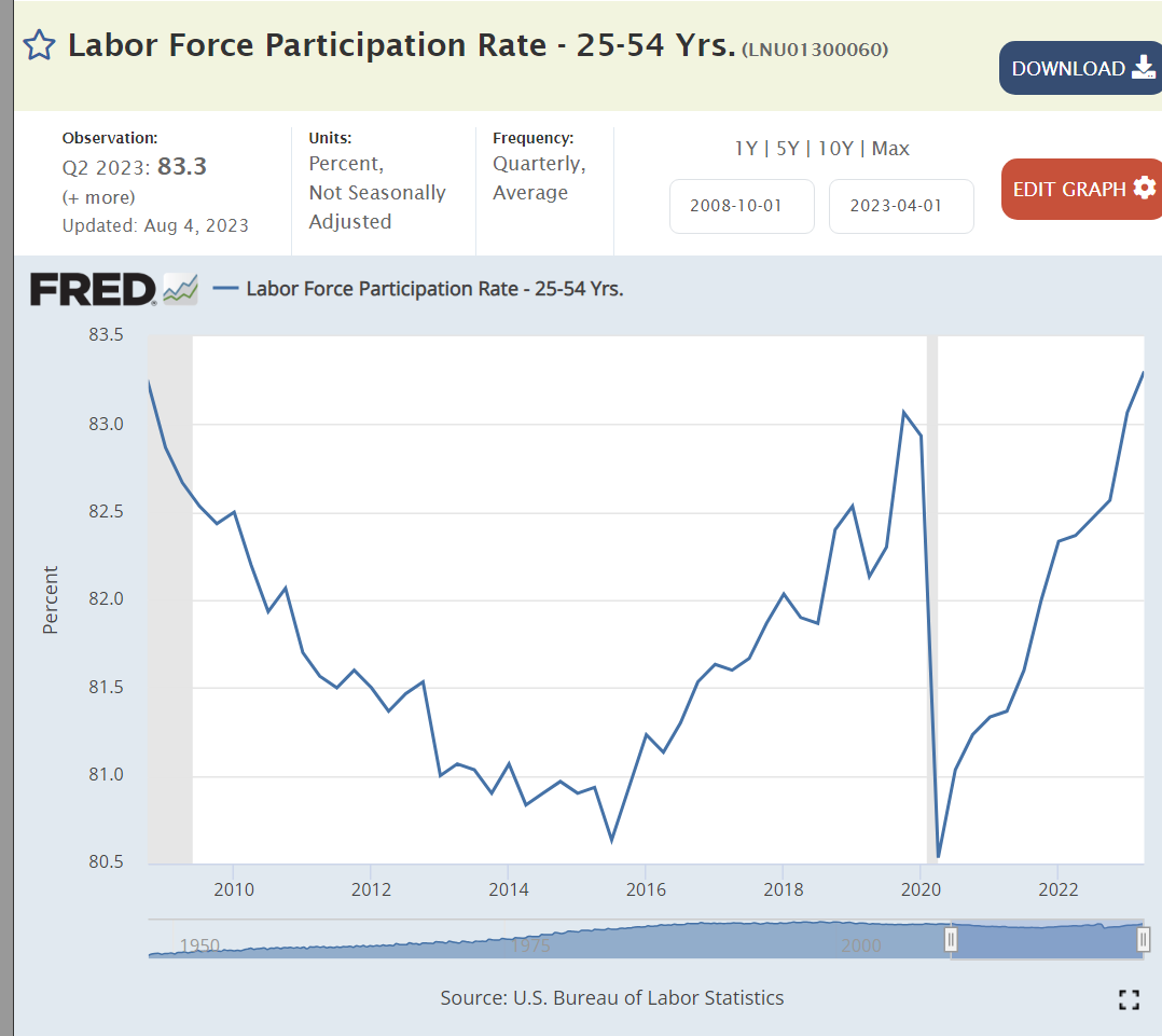
Labor force participation hit record levels after the pandemic and has remained there.
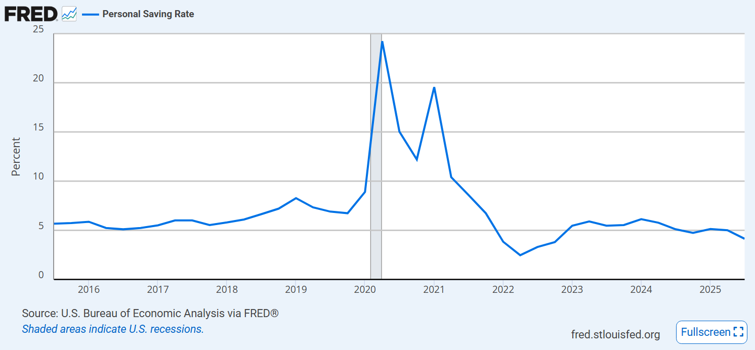
The personal savings rate is low, a bit below the pandemic and trending slightly downward.
Mortgage rates remain elevated, around 6.5%.
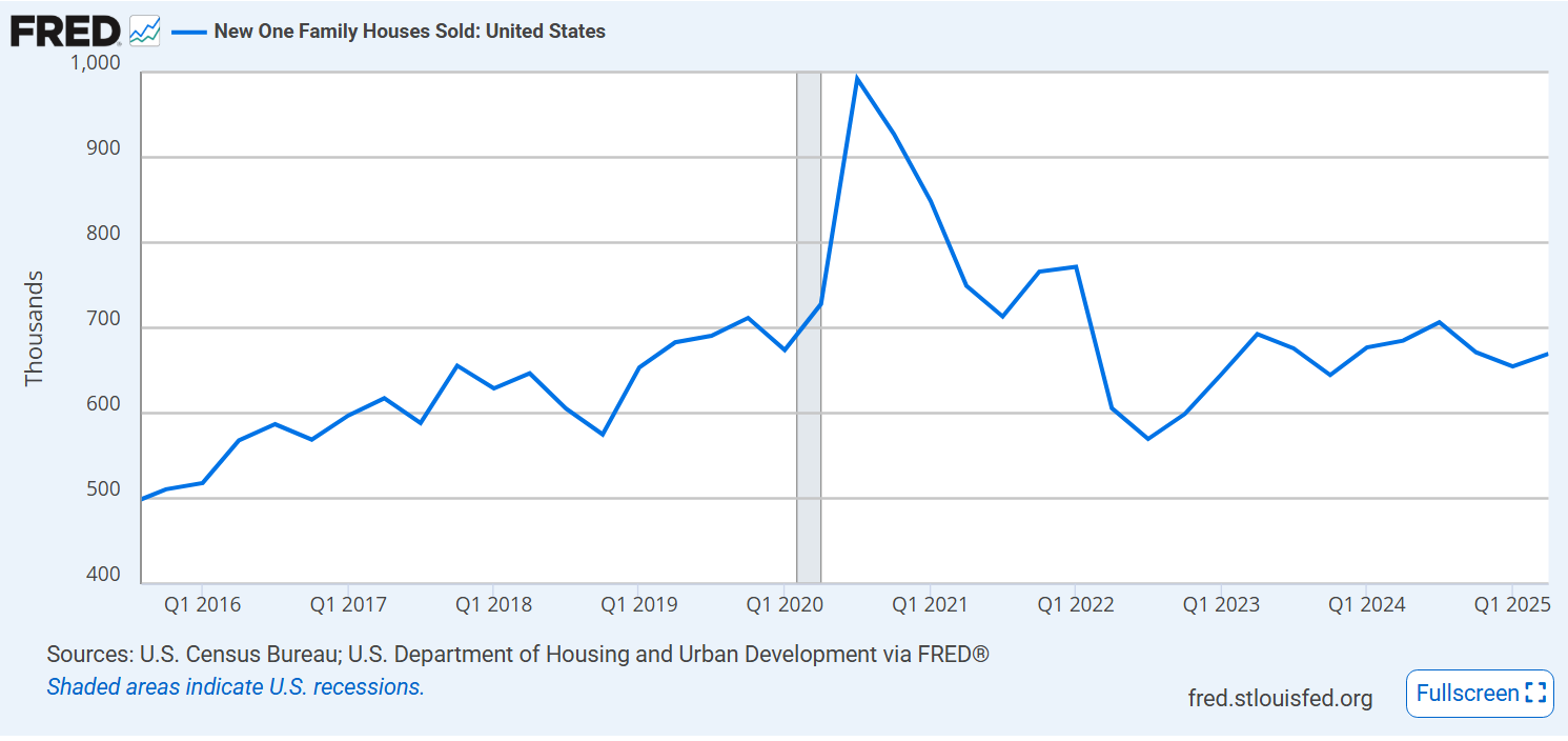
New home sales are pretty stable, at pre-pandemic level.
Housing prices jumped from $320,000 to $440,000 after the pandemic. They have fallen back by 5% in 4 years.
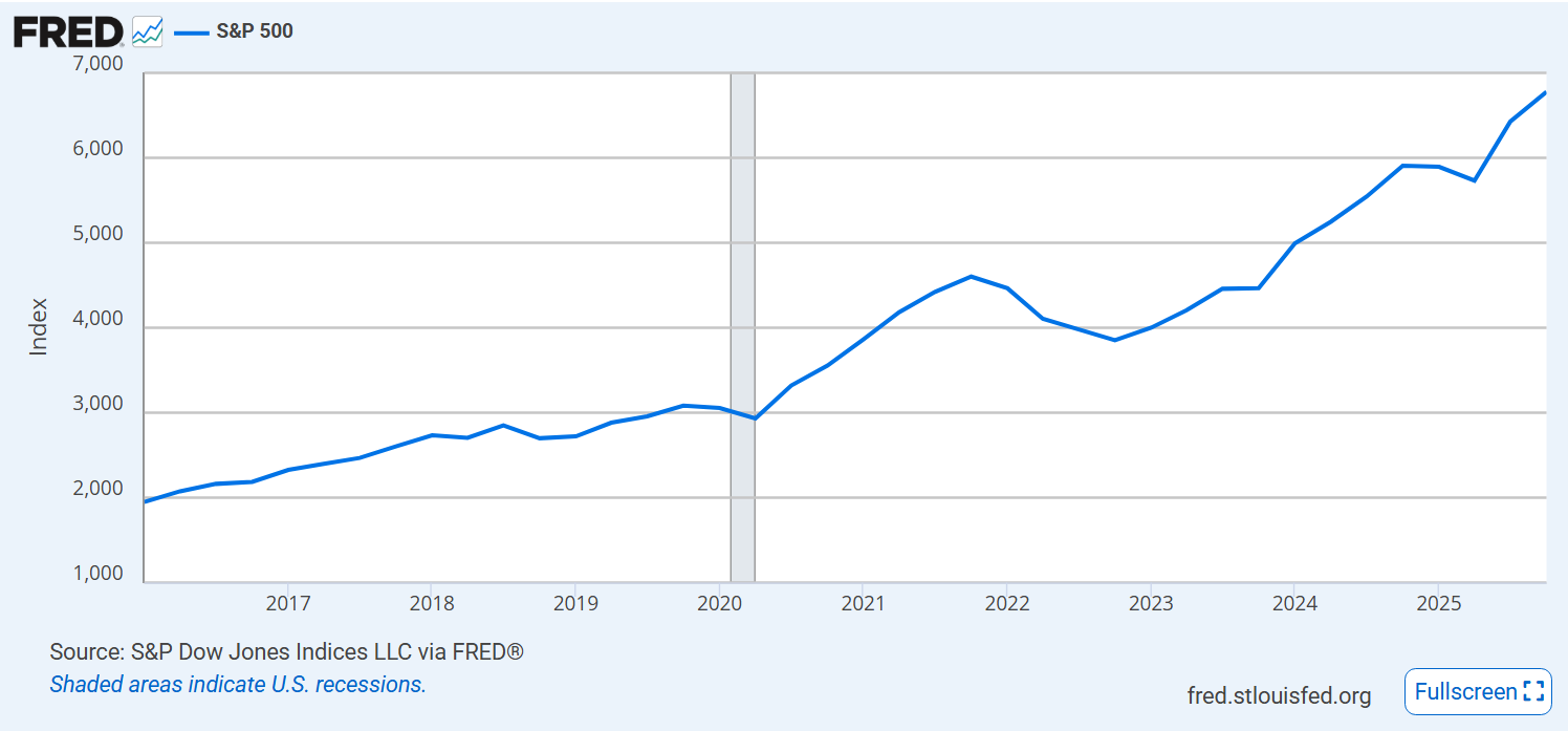
The US stock market continues to climb.
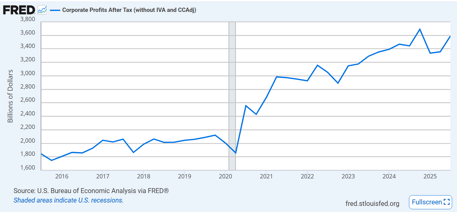
Corporate profits have roughly doubled since before the pandemic.
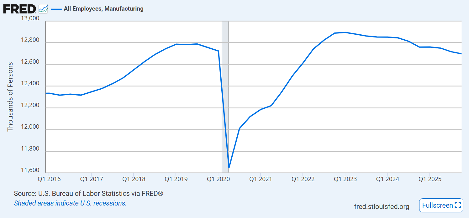
Manufacturing employment continues to decline.
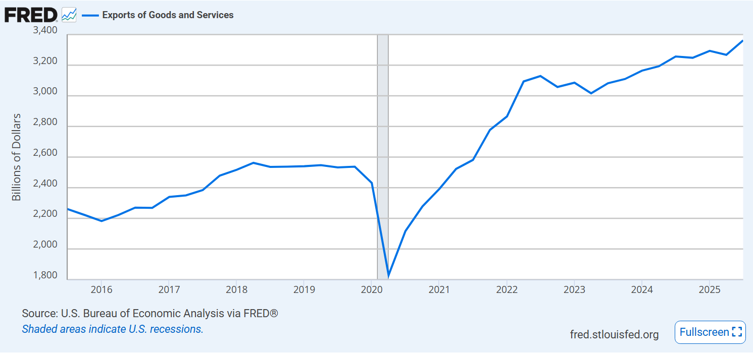
Exports are up 50% and still growing slowly.
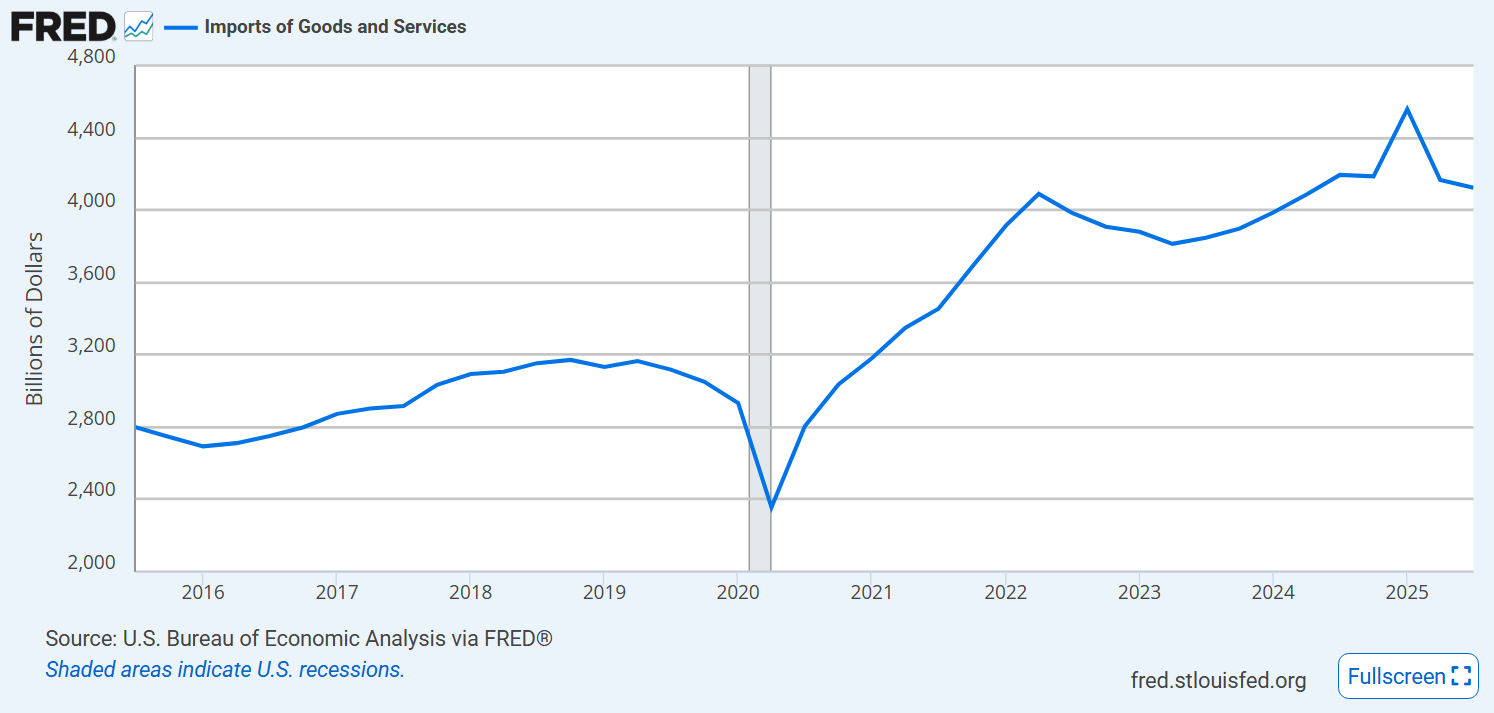
Imports also increased by 50%.
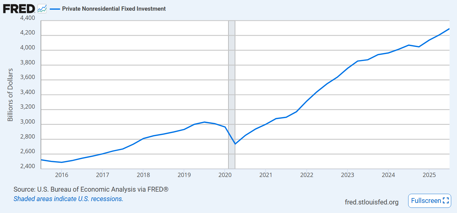
Businesses continue to invest.
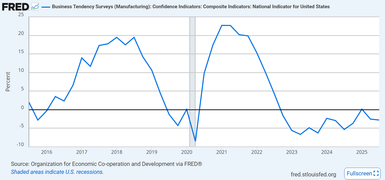
Business confidence remains weak.
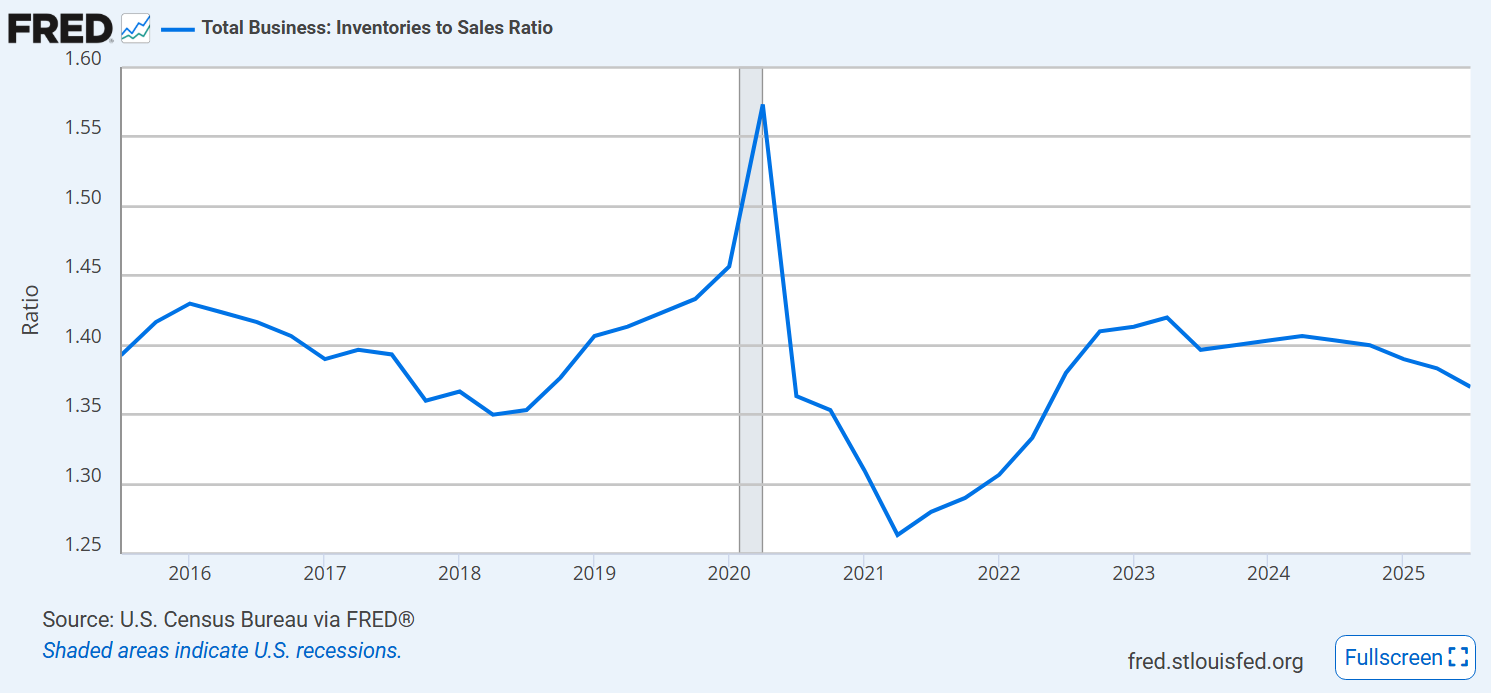
Businesses have maintained their target inventory to sales ratios.
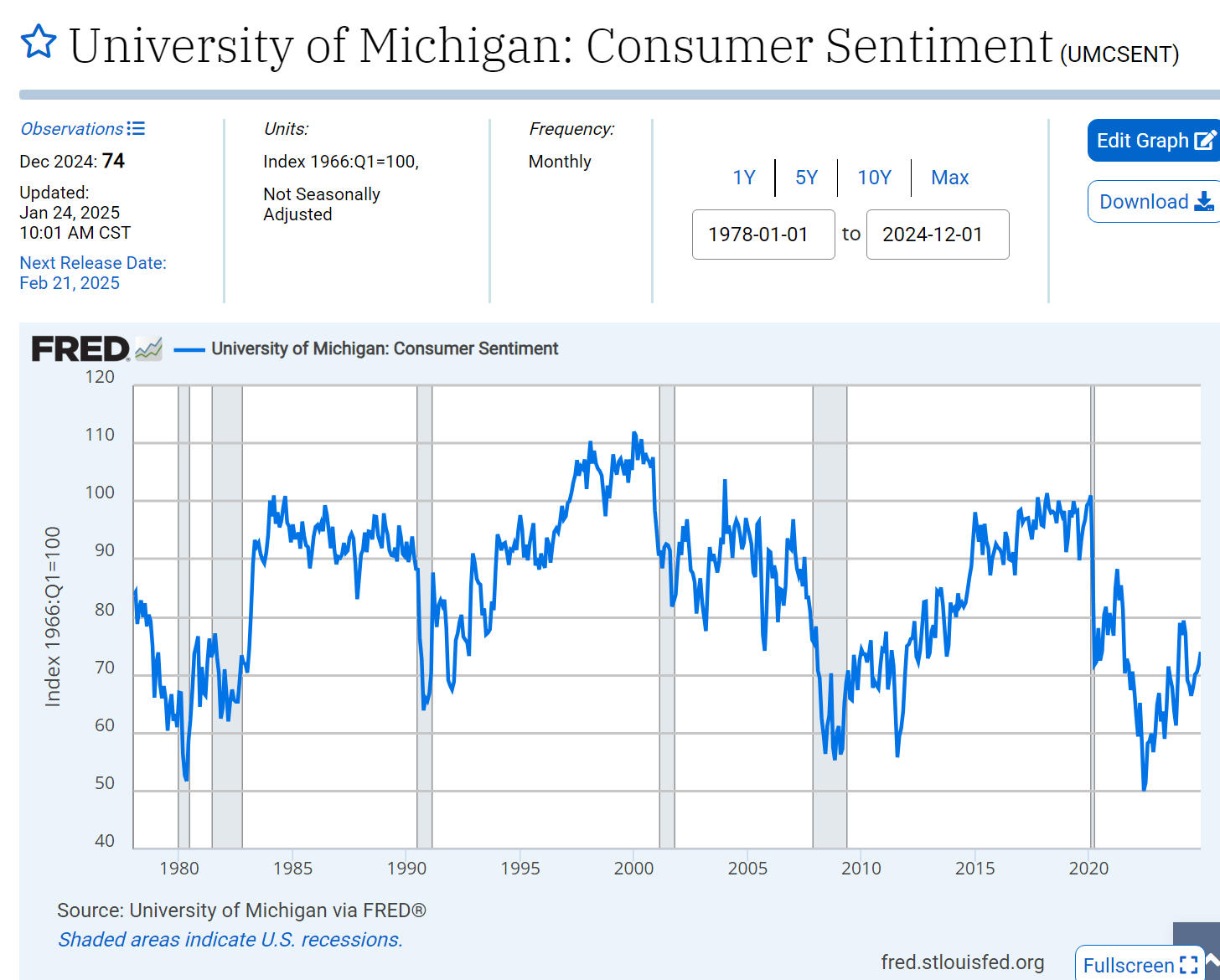
Consumer confidence is down and weak.
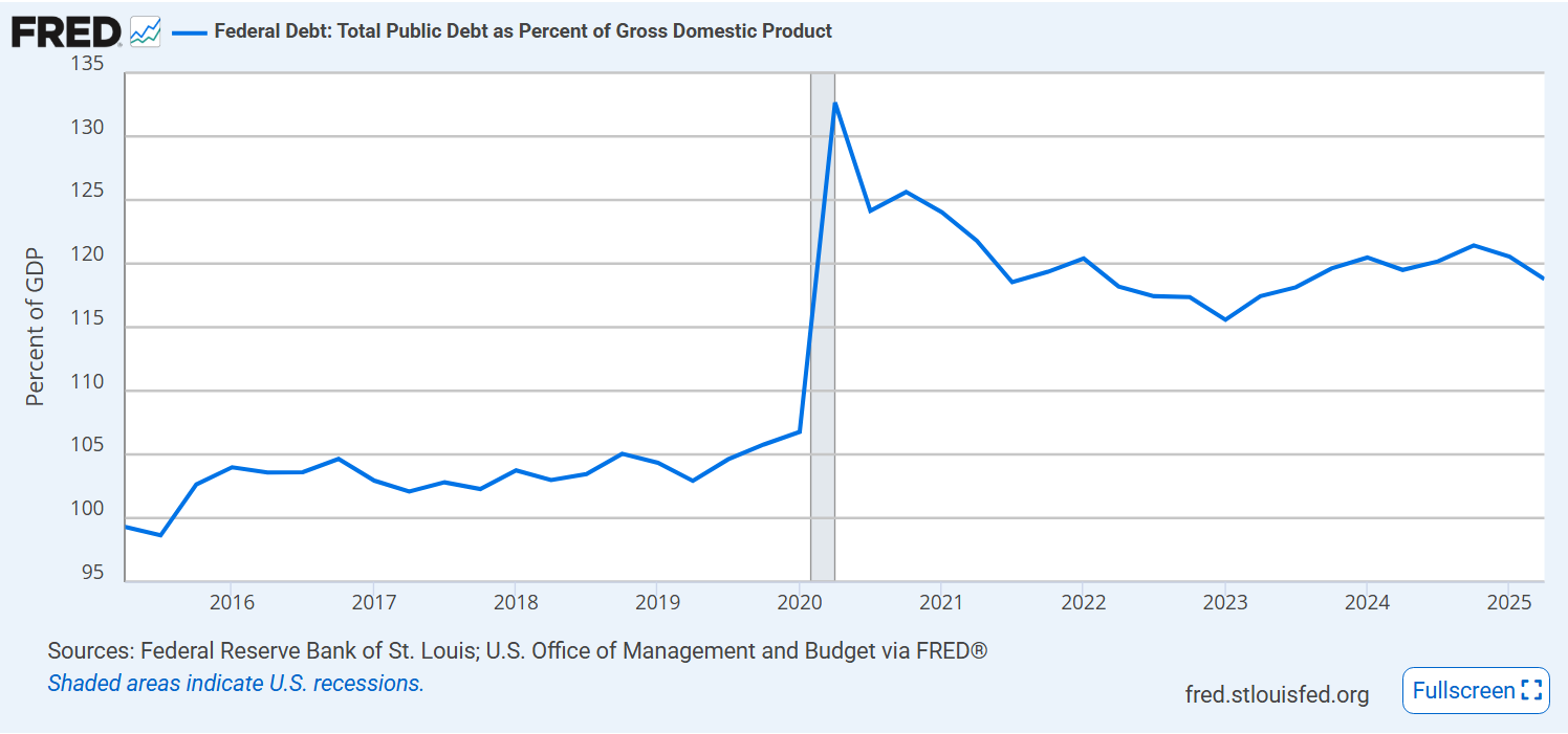
Federal debt % of GDP remains at 120%, up from 105%.
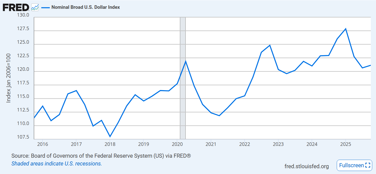
Value of the US dollar increased by 10-12% after the pandemic, but has retreated by 6%.
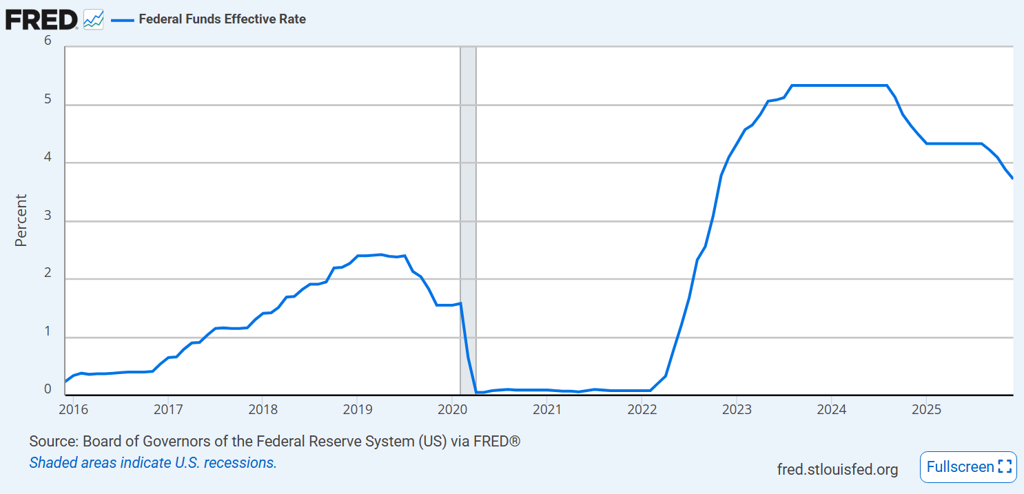
The Federal Reserve Board has reduced interest rates by 1.5%.
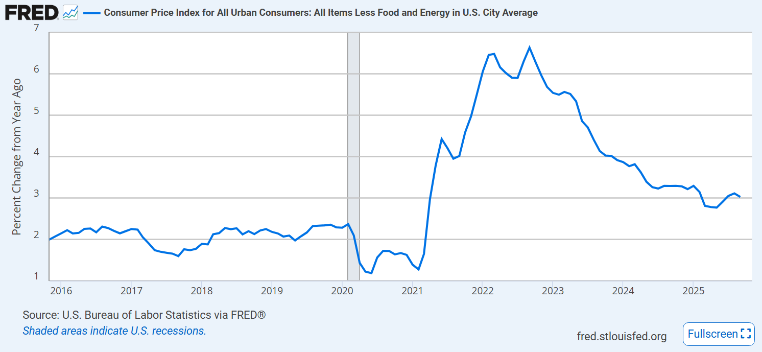
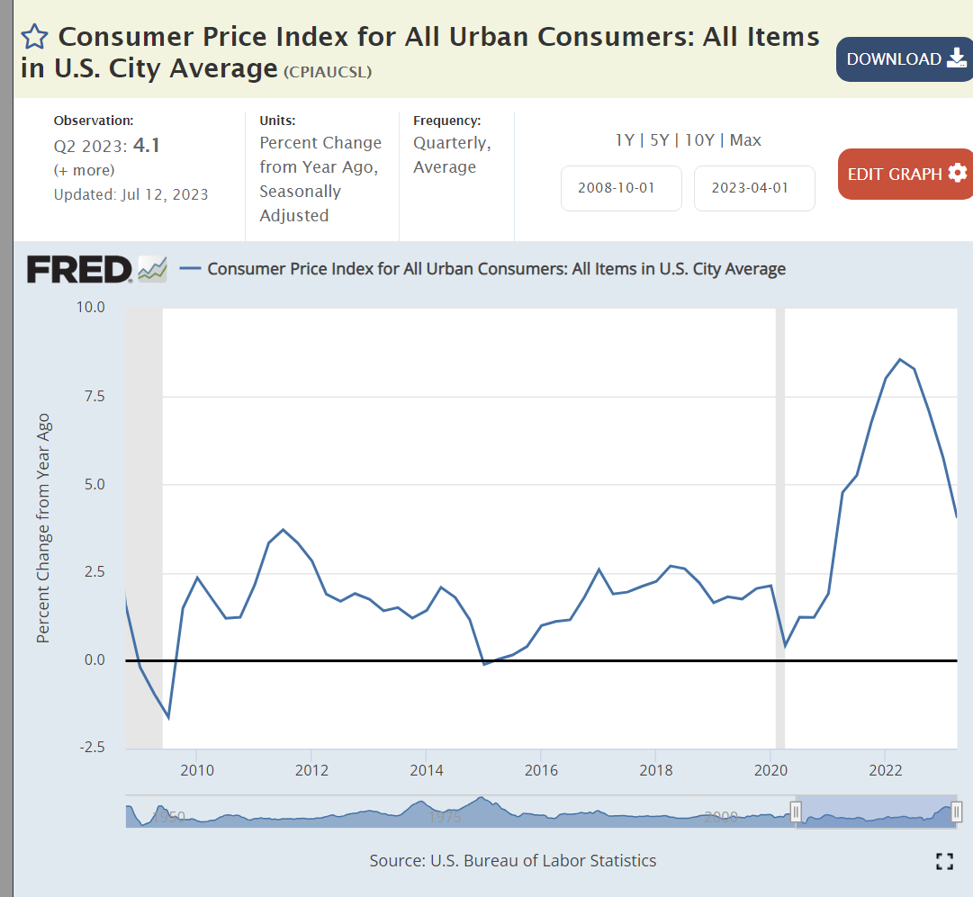
Core inflation rate has levelled off near 3%.
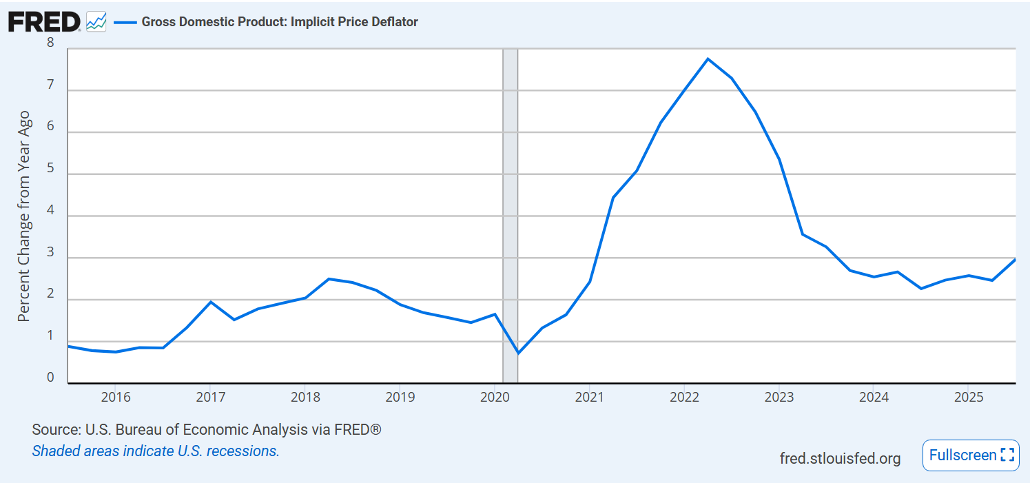
The GDP Price deflator measure of inflation is a little better, approaching 2.5%, but also level or growing.
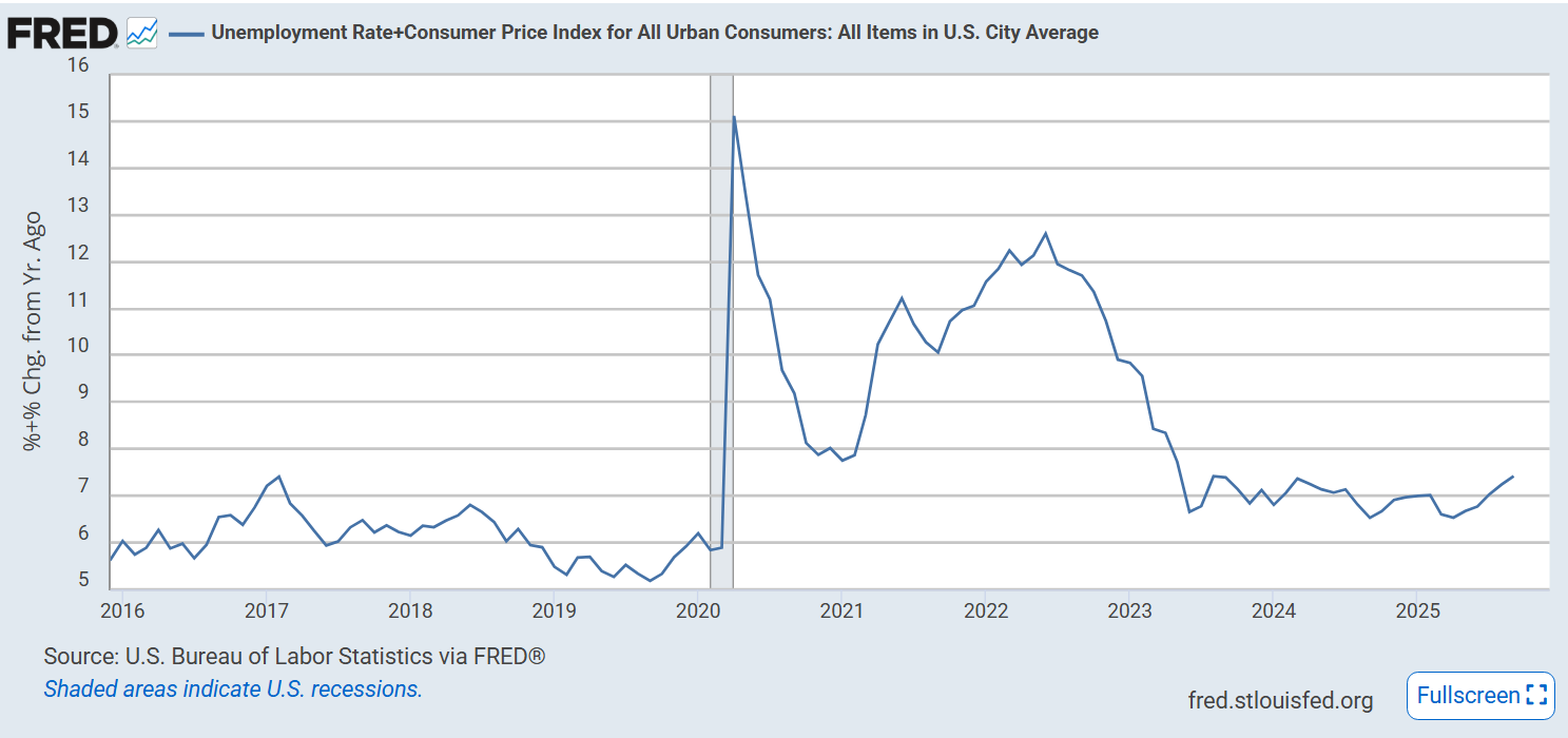
Misery index is up a bit at 7.5%.
Summary
Stock market is solidly up together with corporate profits and business investment.
Inflation and unemployment are up. Budget deficits and debt remain high. Dollar value is down. Manufacturing employment is down. Business and consumer confidence is down.
Other measures are comparable to the 2023-2024 Biden economy base; not improving as often claimed.
The US economy is increasingly resilient and not easily changed by small policy choices or “jawboning”.
We have lost control of our political system and confidence in our institutions. I offer some root cause reasons for this situation in a series of posts. Second post in the series.
Real, inflation adjusted, gross domestic product (GDP) is up 4 and 1/2 times since WWII when the American economy was the savior of Western Civilization and about to invest in the recovery of Europe and Japan. In this long-term perspective, growth is very constant. Critics can point to the capture of a greater share by the wealthy. Optimists can point to the radical improvement in quality not captured by GDP, increased consumer choices available and a larger share of retirees in the population.
Economic Satisfaction Stagnates
Consumer confidence rises with the economy and declines with recessions and polarized politics, but it has no upward trend to match real incomes!
Unlimited Wants, Limited Satisfactions
Economists assume that people have unlimited wants. Most research and common-sense experience show that this is true.
Post-war economists have persistently claimed that Americans “now” have everything they need materially to be happy, but they have been persistently wrong.
Once we have an idea in mind, we tend to consume information that confirms the idea and avoid or deny challenges. Positive, constructive people will be optimists. Others will be pessimists and follow the bad news media.
When we do try to rationally assess our current situation, we compare it with something obvious. It’s usually something prominent, recent, large, and shiny. We compare today with our best ever experience or situation. We reset our expectations to compare with something prominent in our experience. We don’t plot graphs of our real annual earnings, wealth and leisure. Our expectations are anchored in our best experiences. Current expectations tend to move back to a neutral evaluation.
Humans want more. We are rarely satisfied. That means we are easily distracted in the modern world by marketers, influencers, journalists, bloggers and politicians. Human nature has not changed. Our true economic condition has improved with little impact. Our access to information, education, knowledge and wisdom has increased with minor impact. The ability of communicators to influence our perceptions of the world has greatly increased and we have generally not improved our defenses. “We have much, much work to do today” – Mr. Thoburn Dunlap, 1970, Fairport Harbor, Ohio high school teacher.
Hamilton County’s Per Capita Personal Income exceeded $80,000 in 2020.
This ranks above the 97th percentile of the 3,100 U.S. counties.
Hamilton County ranks first in Indiana and would rank first in 30 other states.
Nationally, Hamilton County ranks 42nd among the 600 counties with populations of 100,000+ people. These counties represent 80% of the U.S. population.
Hamilton County’s per capita income is 72% higher than the median county ($46,600) in the U.S.
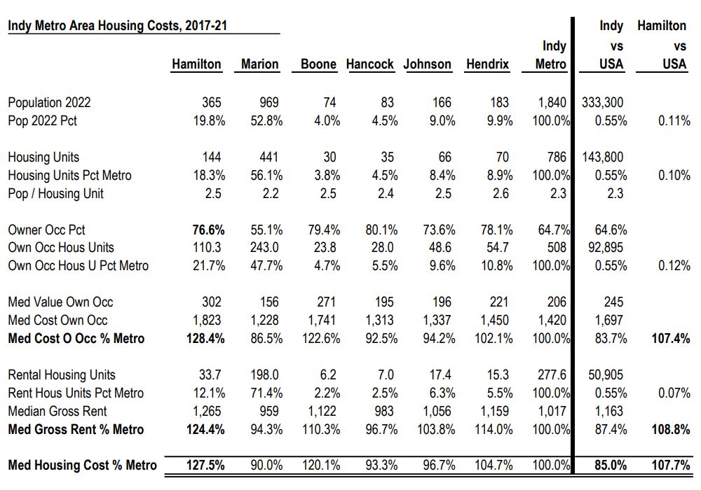
In general, Hamilton County’s costs are similar to those of the Indy metro area. It’s 357,000 residents account for just 17% (1 in 6) of the formal Indy metro area’s 2,075,000.
Solid county level data is not available for all areas, but limited comparisons helped to identify goods and services that might differ between Hamilton County and the Indy average.
Hamilton County’s housing is 8% more expensive than the national average rather than 15-17% lower as seen in metro Indianapolis. The housing stock is also newer, larger and higher quality. The full housing price difference would increase the total cost of living measure by 7%. Considering one-half being due to age/quality and one-half due to prices adds 3.5% to 93.1% to yield a revised 96.6% cost of living ratio.
Indiana local taxes average 9.3% of income versus 10.2% nationally. This 10% savings on a 10% cost factor reduces the overall cost of living measure back down to 95.6%. State sales and income taxes do not vary by county. Hamilton County’s property and income taxes are lower than its large population peer group in Indiana.
Food Prices
Historically, Indianapolis has been a competitive grocery market. Kroger has a leading market share. Cub Foods and Marsh have left the market, but Meijer’s, Trader Joe’s, Whole Foods, Fresh Thyme, Fresh Market and Market District now compete with the others.
Hamilton County’s retail sales per capita figure is 14% above the national average, despite the very high concentration of retail stores in Marion County along 82nd/86th Street. The county is well served by retailers of all kinds.
Food away from home makes up almost 5% of the consumer price index. No restaurant food index is publicly available. However, the Big Mac price in Hamilton County is $4.59 versus the $4.39 national average price, a 5% premium. If this applied to all restaurant prices, the overall cost of living index would be 0.3 higher, 95.9. The average Indiana Big Mac price was just $4.11.
The Economic Policy Institute provides “modest income” food prices that are 19% higher in Hamilton County than in Marion County. Given the proximity of the counties and the long-standing coverage of “food deserts” in Indianapolis contrasted with nearly none in Hamilton County, this indicator is suspect.
Hamilton County has 1.8 hospital beds compared with the national average of 1.9 and the Indiana average of 3.3. It has 1.5 primary care physicians versus 1.0 nationally and 1.3 in Indiana. 10% of Hamilton County households have medical bills in collections compared with 17% nationally and 19% in Indiana. Access to health care is adequate.
The Best Places website uses a simple index of a standard hospital bed night, a doctor’s visit and a dentist’s visit indicating that Hamilton County health care costs are equal to the national average (100).
A Rand Corporation study indicates that Indy metro hospital rates are 25% higher than the national average. This is driving Indiana statehouse political battles with claims and counterclaims. Professional services fees were 25% below the national average.
Although health care is as much as 18% of GDP in the US, the share in the consumer price index is only 5%. If Hamilton County consumer costs are the same as the nation, this would increase the cost-of-living index by 0.6 points to 96.5.
Utilities
Best Places pegs Hamilton County’s utility costs at 93 rather than 107.
Indiana natural gas prices are more than 20% below the 50 state median.
Local utilities are probably at least 10% lower than in the summary statistics, so the COL index should be reduced by 0.9 points based on their share of spending, reducing the index to 95.6.
Transportation
Indiana used car prices are the lowest in the nation, 11% below the average.
The Economic Policy Institute and Indiana Family and Social Services Administration indicate that Hamilton County childcare costs are 13% higher than in Marion. Because childcare accounts for just 0.6% of spending, no adjustment is indicated.
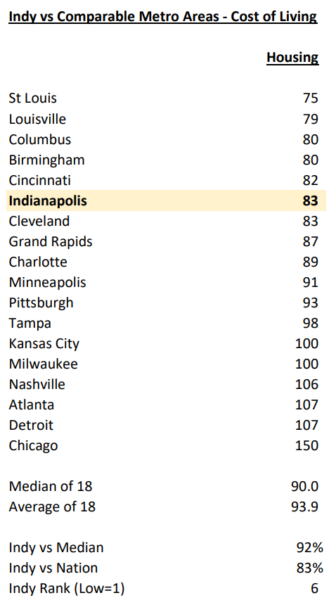
Summary: Hamilton County Costs are 4% Lower than the National Average
County level housing, health care and grocery costs added more than 4% while lower taxes and utility costs subtracted almost 2% for a final score of 95.6, more than 4% below the national average.
The US Census Bureau’s American Community Survey (ACS) is the best publicly available data source for housing data at the county level. The most recent survey covers 2017-21.
The metro Indy area’s housing costs are just 85% of the national average. Hamilton County’s housing costs are 28% higher than the metro average, but only 8% higher than the national average.
Hamilton County’s 40th percentile rent for this period is $1,265, 24% higher than the metro area. The median monthly cost for a homeowner with a mortgage is $1,823, 28% higher than the metro area.
77% of Hamilton County residents own their homes versus 65% in the metro area and in the national average. Hamilton County contains 22% of the owner-occupied homes (110,000) and 12% of the rental units in the metro area (34,000).
The Economic Policy Institute estimates the cost of modest housing in Hamilton County to be 32% above Marion County, less than the 41% indicated by the 128% to 90% ratios to the nation.
The Washington Post reports rental data by county through June, 2023. This also shows a 27% premium between Hamilton County and the weighted average for the 6 main Indy metro counties.
Hamilton County total housing starts have doubled between 2019 and 2022, not as fast as the national average for apartment units, but fast enough to have a cooling impact on rising rental prices.
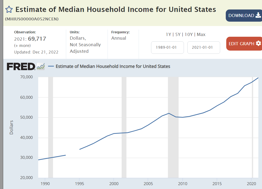
Hamilton County’s $105,000 median household income is 50% higher than the national level of $70,000. The 28% premium of average housing costs is not a significant burden for the median household income family.
On the other hand, families with the $70,000 national median income or lower income do struggle to find affordable housing in the rental and owner occupied housing markets locally.
State and local taxes are mostly driven by the state. In Indiana, state sales and income taxes account for 63% of the total. Local taxes account for 37% of the total.
Indiana is a lower tax state. Various sources rank it 11th to 18th lowest, with a median ranking of 14th. Hoosiers pay 9.3% of their income for taxes.
Indiana’s 9.3% paid is a little higher than 10th rated Oklahoma’s 9.0% and a little less than 25th rated New Mexico’s 10.2%. It is significantly lower than 40th rated Utah’s 12.1%.
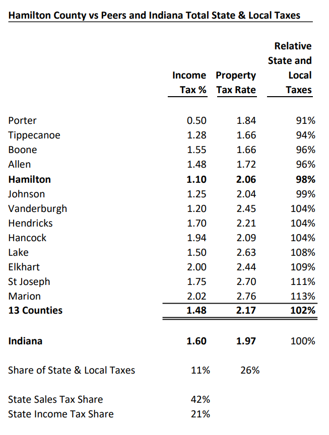
Hamilton County’s 1.1% income tax rate is the 12th lowest of 92 counties in Indiana, 31% lower than the average of 1.6%. The median is 1.75%. Its median property tax rate is 5% higher than the state average. The weighted average total state and local tax rate for Hamilton County is 2% lower than the state average. The Hamilton County total taxes paid as a percent of income is comparable to 12th ranked Louisiana and Florida at 9.1%.
Hamilton County has lower taxes compared with its Indiana peer counties, the top 10 in population plus Indy metro Johnson, Boone and Hancock counties. Its 1.1% income tax rate is lower than all except Porter County; significantly (26%) below the 1.48% average. Its median property tax rate is 5th lowest of the 13, 5% below the peer average. The peer counties’ total tax rate is 2% above the Indiana average. Hamilton County is 2% below the Indiana average.
Real mortage interest rates can be calculated as the difference between nominal mortage interest rates and the 10-year Treasury Bond interest rate. Although nominal interest rates have ranged from 3% to 16%, the real, after expected inflation, interest rates are remarkably consistent, averaging just 1.7% and ranging between 1.3% and 2.1% in 70% of the last 52 years. The peak real rate was 3.0% in 1982 following the unexpectedly high and remaining high nominal rates of the prior 4 years.
Banks, mortgage-backed securities investors and mortgage borrowers all take risks when they complete mortgage transactions. Lenders are betting that their present and future borrowing interest rates are and will be low enough to fund their mortgages at a profit. Each lender locks in funding commitments for a reasonable share of the loan life and counts on the consistency of interest rates over the business cycle to fund the remaining portion. Lenders that experience a mismatch put their stockholders’ equity at risk and face bankruptcy. Investors in mortgage-backed securities are subject to valuation change risks throughout the period in which they are invested. Most such investors hold diversified portfolios of mortgages (region, amount, riskiness, urban vs suburban vs rural) and non-mortgage assets to ensure that any investment decision will not be too damaging.
Fixed-rate mortgage borrowers are betting that inflation will not fall too much lower than the expected inflation rates when they borrowed. If so, they will be paying back the mortgage in higher real value dollars than expected. If inflation and mortgage rates drop by more than 2%, most borrowers will seek to refinance their mortgages at the new, lower market rates, paying another round of closing costs for this privilege. Fixed rate borrowers are also hoping that inflation will be higher than the expected inflation rates at the time they borrowed, allowing them to pay back their debt with cheaper real dollars. Mortgage originators do not generally have the legal right to “call” the debt and require a change in the rates and terms as many commercial lenders and bond issuers do.
The “good news” is that the US mortgage market is very efficient and the real interest rate premium for borrowing to own a home is just 2% more than what the US government pays for borrowing. Borrowers face interest rate change risks, especially being caught with a high interest rate mortgage when inflation rates fall if they are unable to refinance.
The market has been tested through 7 business cycles and held up very well. The “Great Recession” exposed excessive risk taking by mortgage originators and funders. They lost money and many went out of business. Riskier mortgages are rarely issued today, and government regulations provide some added protection against any future overreach.
For higher income households that itemize deduction on their federal tax returns, the nominal interest rate paid is a tax-deductible offset to earned income. These individuals typically pay 22%, 24% or 34% marginal tax rates. A 5% nominal tax rate can provide a 1%, 1.25% or 1.65% reduction in the effective interest rate, thereby making the 2% real mortgage rate less than 1%. Higher income households can benefit greatly from this tax benefit.
Real, after inflation, Gross Domestic Product is up by one-third, despite the pandemic. That’s 2% annually, despite the Great Recession and the pandemic. The US economy is very solid.
A 21% increase in per capita income during this time. Quite solid and constant growth.
Inflation averaged a bit less than 2% before the pandemic, spiked to 8%, and has since declined to 4%. Experts disagree on whether it will return to 2% soon.
Gas prices are the most obvious component of inflation. They are largely driven by global supply and demand. Prices today are the same as in 2011-14, despite the general inflation increase of more than 20% since then.
Despite the pandemic, US unemployment is at a 50 year low!
Job seekers today encounter 3 times as many job openings.
Core age labor force participation has snapped back after the pandemic.
Investment values have doubled.
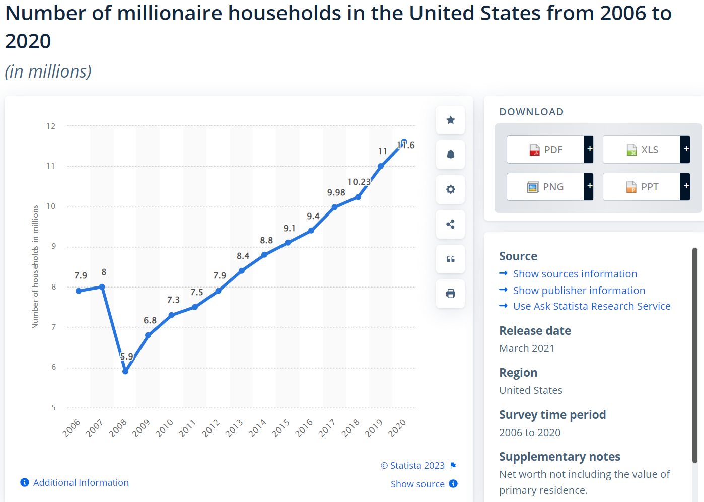
The number of millionaires and billionaires in the US has continued to increase.
Personal savings rates rose from 6% to 9% before the pandemic, shot up and fell back down to just 4% recently.
Housing values have doubled since the Great Recession.
Mortgage rates averaged 4% after the Great Recession, dropped to 3% and then increased to 6%+ as the Federal Reserve raised interest rates.
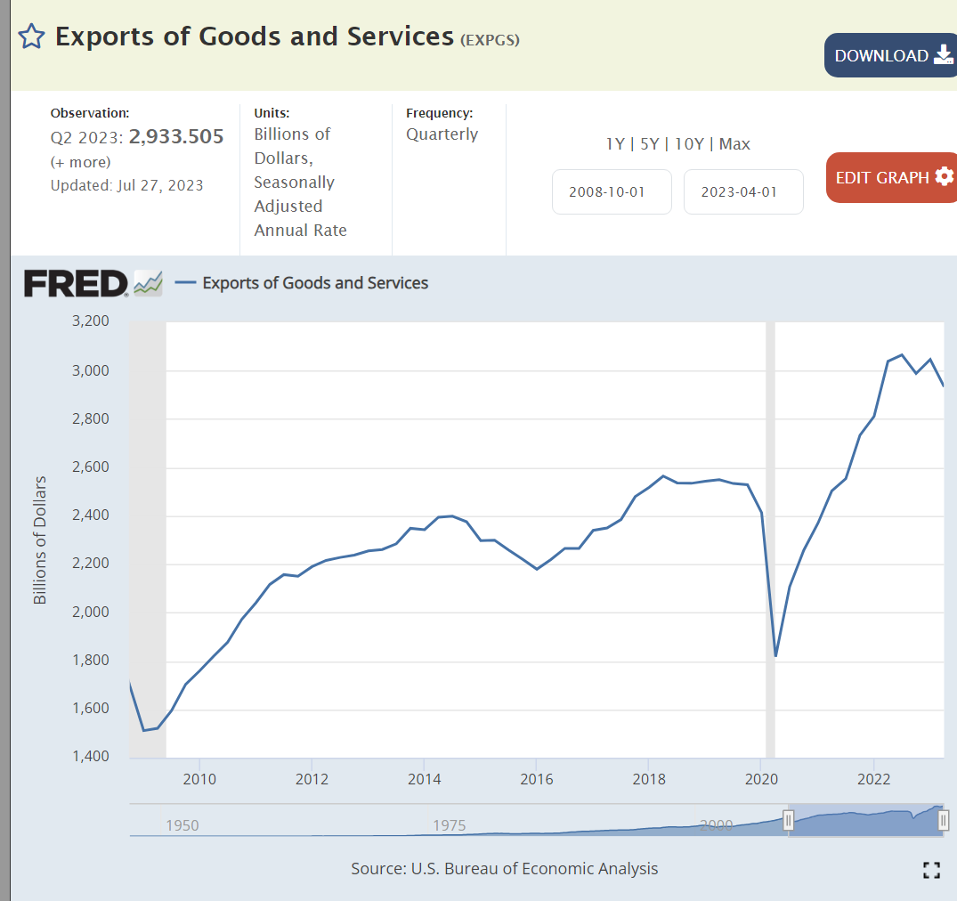
US exports have nearly doubled in 14 years.
Despite the Trump tariffs, which Biden has maintained, imports have also nearly doubled.
Despite historically slower growth rates, higher budget deficits and looser monetary policies, the US dollar is more highly valued today than in 2008.
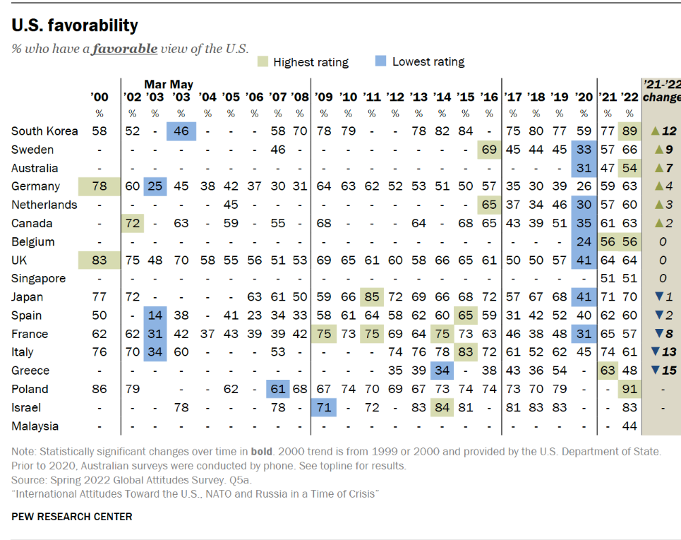
Foreign countries still see the US as a positive ally, despite their concerns during the Trump era.
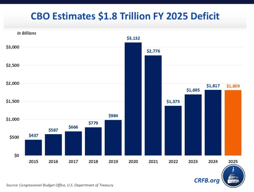
Obama returned the budget deficit to a “reasonable” 3% by 2016. Trump expanded it to 5% and then 15% as the pandemic struck. Biden drove some recovery to 5% by 2022, but has not driven further reductions.
US coal production is in a long-term decline.
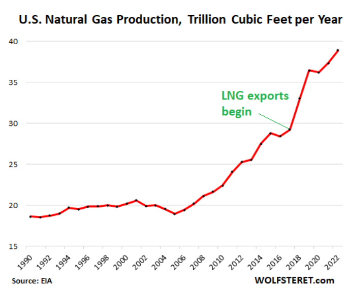
Natural gas production has nearly doubled in 14 years.
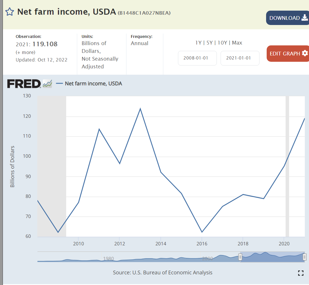
Net farm income has been significantly above the base for 6 of the last 14 years, despite lavish Trump farm subsidies.
Manufacturing employment has continued to rise slowly in the last 14 years against the headwinds of international competition.
It’s difficult to put the pandemic in perspective, but here we see a 2-year reduction in expected lifespans. Opioid deaths and so-called “deaths of despair”, alcohol, drugs, suicide, also play a role.
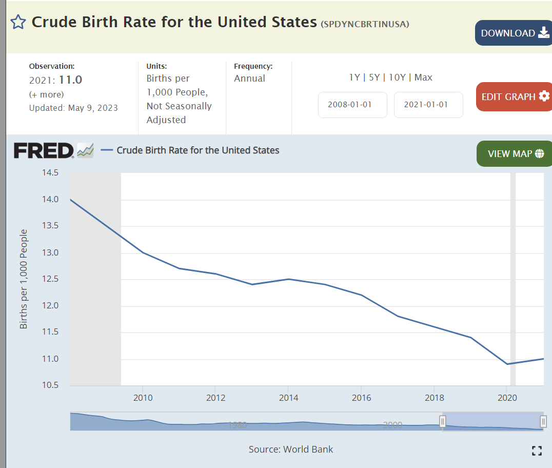
Birth rates continue to drift lower as seen in all regions of the world.
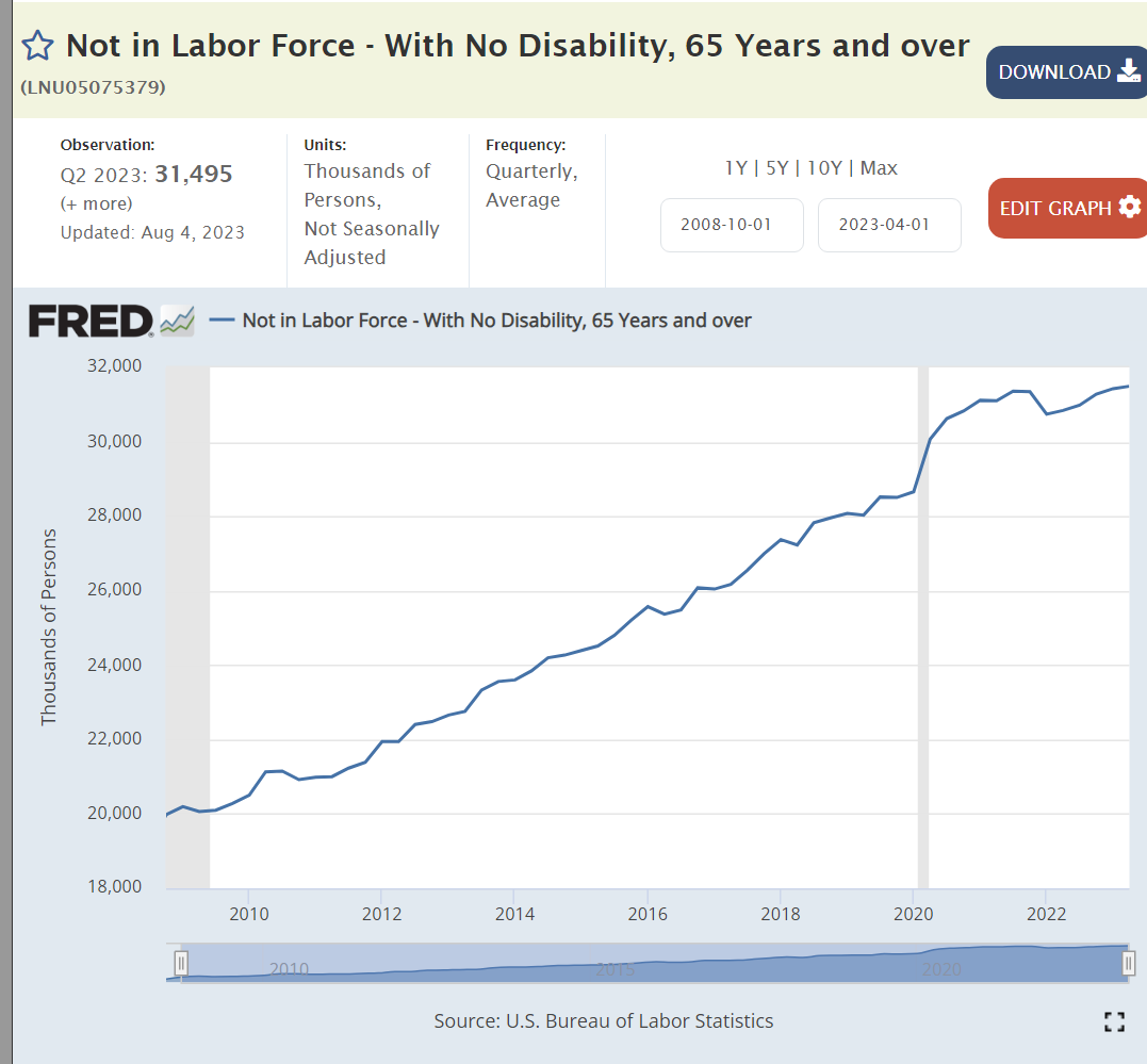
The number of retirees has increased by more than 50%.
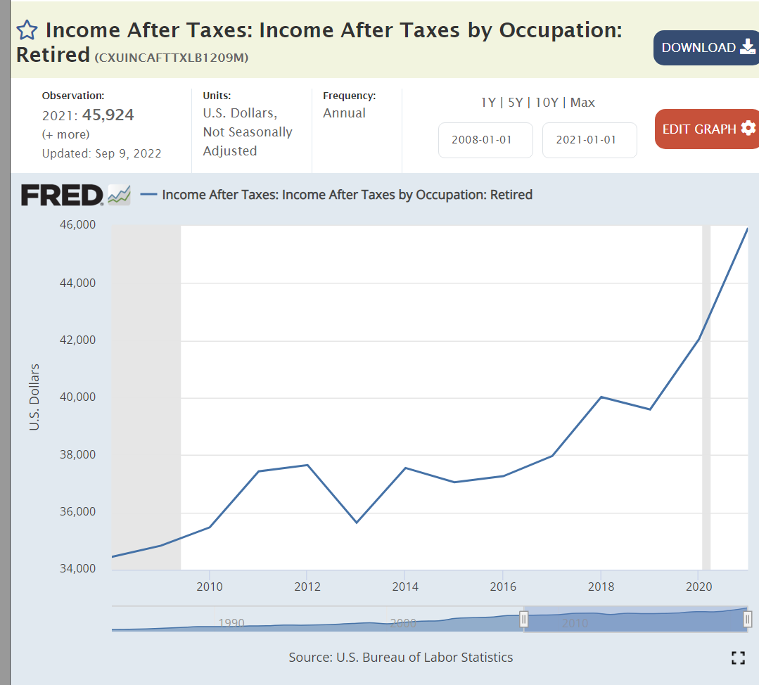
Retiree incomes are up by one-third, matching inflation.
Prospective retirees have doubled their cumulative savings.
The abortion rate has continued to fall in the last 30 years.
Church attendance has dropped from 40% to 30%.
Summary
The US economy recovered slowly after the Great Recession and then very quickly after the pandemic. Real, after inflation, output and per capita output increased. The labor market became very tight. Asset prices (investments and housing) rose for intrinsic and monetary reasons. The US remained a competitive international producer. The federal budget deficit was better at the end of the Obama period but worse for Trump and Biden. The pandemic reduced life expectancy and households had fewer children. Successful retirements grew and will grow. Social trends continue, uninterrupted by political positioning and policies.
Perceptions of the country and the economy are increasingly shaped by partisan political party views. Nonetheless, the US economy continues to grow and thrive.
Franchising provides an opportunity for qualified individuals to own a business and earn equity-like rewards, without outstanding industry expertise, with lower business failure risk, requiring relatively modest equity investments and the opportunity for advantageous bank and small business loans.
Franchising provides the owner of a product or service concept with the opportunity to expand using “other people’s money”. It facilitates geographic and international expansion leveraging locally knowledgeable managers/investors. It allows differentiated products, services and systems to be replicated quickly and consistently. It provides legal agreements that ensure that the franchisor’s brand is enhanced and not damaged by the franchisee’s operations. It provides a system that strongly aligns the interests of local managers/owners with those of the central business.
History
Franchising has experienced several “boom and bust” periods, fraudulent deals and changing relations between franchisors and franchisees through time. Initial growth began in the 1850-1920 period together with the growth of the manufacturing and transportation industries. Automobiles, farm equipment, sewing machines, service stations, auto parts, pharmacies, soft drinks and train stop/car hop restaurants lead the way originally using the product franchising model. The depression interrupted the growth of franchising. Automobile dealers, service stations and soft drink distributors accounted for 80% of franchising before the depression.
Franchising accelerated again after WWII with fast-food restaurants leading the way, accompanied by a diverse set of laundry, hotel, rental car, real estate and convenience stores. These businesses were often still tied to products or patented equipment. However, McDonalds (1955) offered the first business format franchises which provided greater opportunities in a growing, travelling society.
Business format franchising “includes not only the product, service, and trademark, but the entire business format itself: a marketing strategy and plan, operating manuals and standards, quality control, and a continuing process of assistance and guidance.”
With rapid growth came accounting fraud by franchisors, one-sided contracts, overlapping deals, pyramid schemes and conflicts between franchisors and franchisees. The Energy Crisis of the 1970’s bankrupted a large share of service stations. State and federal regulations enacted in the 1970’s ensured that standard disclosure agreements were used, allowing potential franchise owners to work with their lawyers to ensure that they understood the deals they were making.
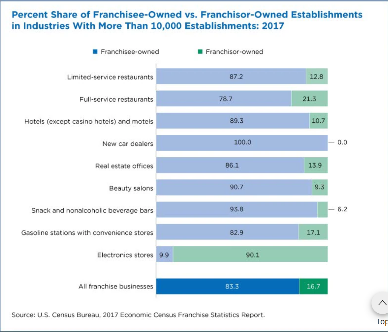
Data on the franchising industry is not standardized. Two industry associations and the US Census Bureau provide somewhat inconsistent data. Nonetheless, the growth of franchising after the “bust” in the 1970’s is amazing. The number of establishments has grown from 375,000 (1973) to 420,000 (1988) to 530,000 (1990) to 775,000 (2021). Total employment has grown more slowly, from 7 million (1988) to almost 10 million (2017). Sales has grown much faster from $160 billion (1975) to $350 billion (1980) to $530 billion (1985) to $1 trillion (2004) to $1.3 trillion (2007) to $1.5 trillion (2012) to $1.7 trillion (2017).
Leading sectors by annual earnings include senior care ($155K), real estate ($153K), personal services ($126K), business services ($122K) and pet services ($119K).
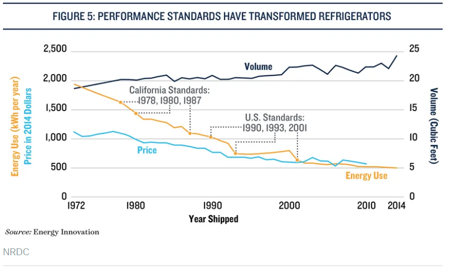
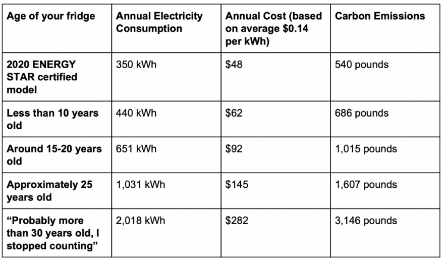
The US Dept of Labor does not publish a consumer price index specifically for refrigerators, but the category it belongs in showed essentially zero nominal inflation between 1994 and 2018. The real price decline shown in the first chart probably continued through 2018.
Refrigerators and appliance prices spiked by more than 10% in 2021 as consumer demand for durable goods grew 20% during the pandemic, supported by government transfer payments.
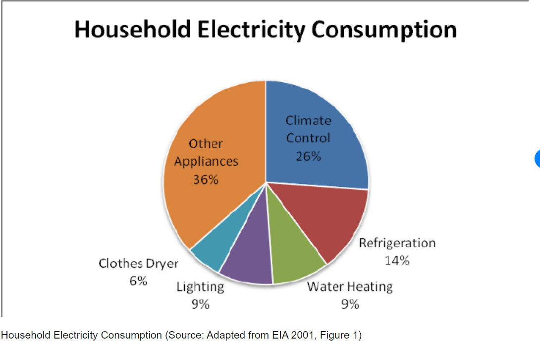
Refrigerators now account for just 7% of home electricity consumption, down from 14% in 2001.
Opinion writers differ on who gets credit for the improved price/performance results for refrigerators, but it seems clear that both energy standards and inventive firms share credit.